AI Acceleration
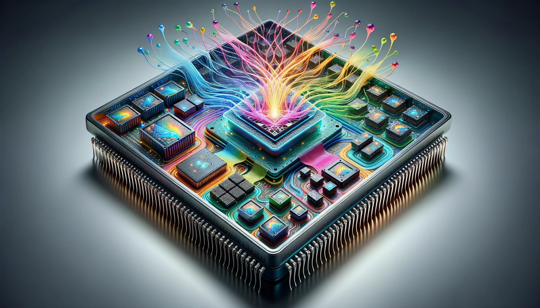
DALL·E 3 Prompt: Create an intricate and colorful representation of a System on Chip (SoC) design in a rectangular format. Showcase a variety of specialized machine learning accelerators and chiplets, all integrated into the processor. Provide a detailed view inside the chip, highlighting the rapid movement of electrons. Each accelerator and chiplet should be designed to interact with neural network neurons, layers, and activations, emphasizing their processing speed. Depict the neural networks as a network of interconnected nodes, with vibrant data streams flowing between the accelerator pieces, showcasing the enhanced computation speed.
Purpose
What makes specialized hardware acceleration not just beneficial but essential for practical machine learning deployment, and why does this represent a fundamental shift in how we approach computational system design?
Practical machine learning systems depend entirely on hardware acceleration. Without specialized processors, computational demands remain economically and physically infeasible. General-purpose CPUs achieve only 100 GFLOPS1 for neural network operations (Sze et al. 2017a), while modern training workloads require trillions of operations per second, creating a performance gap that traditional scaling cannot bridge. Hardware acceleration transforms computationally impossible tasks into practical deployments, enabling entirely new application categories. Engineers working with modern AI systems must understand acceleration principles to harness 100-1000\(\times\) performance improvements that make real-time inference, large-scale training, and edge deployment economically viable.
1 GFLOPS (Giga Floating-Point Operations Per Second): A measure of computational throughput representing one billion floating-point operations per second. TOPS (Tera Operations Per Second) represents one trillion operations per second, typically used for integer operations in AI accelerators.
Learning Objectives
Trace the evolution of hardware acceleration from floating-point coprocessors to modern AI accelerators and explain the architectural principles driving this progression
Classify AI compute primitives (vector operations, matrix multiplication, systolic arrays) and analyze their implementation in contemporary accelerators
Evaluate memory hierarchy designs for AI accelerators and predict their impact on performance bottlenecks using bandwidth and energy consumption metrics
Design mapping strategies for neural network layers onto specialized hardware architectures, considering dataflow patterns and resource utilization trade-offs
Apply compiler optimization techniques (graph optimization, kernel fusion, memory planning) to transform high-level ML models into efficient hardware execution plans
Compare multi-chip scaling approaches (chiplets, multi-GPU, distributed systems) and assess their suitability for different AI workload characteristics
Critique common misconceptions about hardware acceleration and identify potential pitfalls in accelerator selection and deployment strategies
AI Hardware Acceleration Fundamentals
Modern machine learning systems challenge the architectural assumptions underlying general-purpose processors. While software optimization techniques examined in the preceding chapter provide systematic approaches to algorithmic efficiency through precision reduction, structural pruning, and execution refinements, they operate within the constraints of existing computational substrates. Conventional CPUs achieve utilization rates of merely 5-10% when executing typical machine learning workloads (Gholami et al. 2024), due to architectural misalignments between sequential processing models and the highly parallel, data-intensive nature of neural network computations.
This performance gap has driven a shift toward domain-specific hardware acceleration within computer architecture. Hardware acceleration complements software optimization, addressing efficiency limitations through architectural redesign rather than algorithmic modification. The co-evolution of machine learning algorithms and specialized computing architectures has enabled the transition from computationally prohibitive research conducted on high-performance computing systems to ubiquitous deployment across diverse computing environments, from hyperscale data centers to resource-constrained edge devices.
Hardware acceleration for machine learning systems sits at the intersection of computer systems engineering, computer architecture, and applied machine learning. For practitioners developing production systems, architectural selection decisions regarding accelerator technologies encompassing graphics processing units, tensor processing units, and neuromorphic processors directly determine system-level performance characteristics, energy efficiency profiles, and implementation complexity. Deployed systems in domains such as natural language processing, computer vision, and autonomous systems demonstrate performance improvements spanning two to three orders of magnitude relative to general-purpose implementations.
This chapter examines hardware acceleration principles and methodologies for machine learning systems. The analysis begins with the historical evolution of domain-specific computing architectures, showing how design patterns from floating-point coprocessors to graphics processing units inform contemporary AI acceleration strategies. We then address the computational primitives that characterize machine learning workloads, including matrix multiplication, vector operations, and nonlinear activation functions, and analyze the architectural mechanisms through which specialized hardware optimizes these operations via innovations such as systolic array architectures and tensor processing cores.
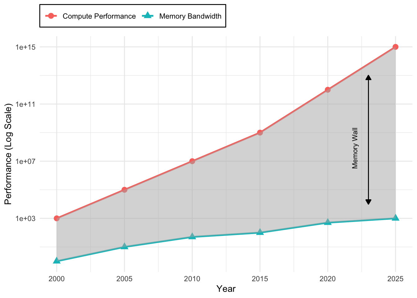
Memory hierarchy design plays a critical role in acceleration effectiveness, given that data movement energy costs typically exceed computational energy by more than two orders of magnitude. This analysis covers memory architecture design principles, from on-chip SRAM buffer optimization to high-bandwidth memory interfaces, and examines approaches to minimizing energy-intensive data movement patterns. We also address compiler optimization and runtime system support, which determine the extent to which theoretical hardware capabilities translate into measurable system performance.
The chapter concludes with scaling methodologies for systems requiring computational capacity beyond single-chip implementations. Multi-chip architectures, ranging from chiplet-based integration to distributed warehouse-scale systems, introduce trade-offs between computational parallelism and inter-chip communication overhead. Through detailed analysis of contemporary systems including NVIDIA GPU architectures, Google Tensor Processing Units, and emerging neuromorphic computing platforms, we establish the theoretical foundations and practical considerations necessary for effective deployment of AI acceleration across diverse system contexts.
Evolution of Hardware Specialization
Computing architectures follow a recurring pattern: as computational workloads grow in complexity, general-purpose processors become increasingly inefficient, prompting the development of specialized hardware accelerators. The need for higher computational efficiency, reduced energy consumption, and optimized execution of domain-specific workloads drives this transition. Machine learning acceleration represents the latest stage in this ongoing evolution, following a trajectory observed in prior domains such as floating-point arithmetic, graphics processing, and digital signal processing.
This evolutionary progression provides context for understanding how modern ML accelerators including GPUs with tensor cores (specialized units that accelerate matrix operations), Google’s TPUs2, and Apple’s Neural Engine emerged from established architectural principles. These technologies enable widely deployed applications such as real-time language translation, image recognition, and personalized recommendations. The architectural strategies enabling such capabilities derive from decades of hardware specialization research and development.
2 TPU Origins: Google secretly developed the Tensor Processing Unit (TPU) starting in 2013 when they realized CPUs couldn’t handle the computational demands of their neural networks. The TPUv1, deployed in 2015, delivered 15-30\(\times\) better performance per watt than contemporary GPUs for inference. This breakthrough significantly changed how the industry approached AI hardware, proving that domain-specific architectures could dramatically outperform general-purpose processors for neural network workloads.
Hardware specialization forms the foundation of this transition, enhancing performance and efficiency by optimizing frequently executed computational patterns through dedicated circuit implementations. While this approach yields significant gains, it introduces trade-offs in flexibility, silicon area utilization, and programming complexity. As computing demands continue to evolve, specialized accelerators must balance these factors to deliver sustained improvements in efficiency and performance.
The evolution of hardware specialization provides perspective for understanding modern machine learning accelerators. Many principles that shaped the development of early floating-point and graphics accelerators now inform the design of AI-specific hardware. Examining these past trends offers a framework for analyzing contemporary approaches to AI acceleration and anticipating future developments in specialized computing.
Specialized Computing
The transition toward specialized computing architectures stems from the limitations of general-purpose processors. Early computing systems relied on central processing units (CPUs) to execute all computational tasks sequentially, following a one-size-fits-all approach. As computing workloads diversified and grew in complexity, certain operations, especially floating-point arithmetic, emerged as performance bottlenecks that could not be efficiently handled by CPUs alone. These inefficiencies prompted the development of specialized hardware architectures designed to accelerate specific computational patterns (Flynn 1966).
Flynn, M. J. 1966. “Very High-Speed Computing Systems.” Proceedings of the IEEE 54 (12): 1901–9. https://doi.org/10.1109/proc.1966.5273.
3 Intel 8087 Impact: The 8087 coprocessor cost hundreds of dollars (up to $700-795 according to various accounts, about $2,100-2,400 today) but transformed scientific computing. CAD workstations that took hours for complex calculations could complete them in minutes. This success created the entire coprocessor market and established the economic model for specialized hardware that persists today: charge premium prices for dramatic performance improvements in specific domains.
Fisher, Lawrence D. 1981. “The 8087 Numeric Data Processor.” IEEE Computer 14 (7): 19–29. https://doi.org/10.1109/MC.1981.1653991.
One of the earliest examples of hardware specialization was the Intel 8087 mathematics coprocessor3, introduced in 1980. This floating-point unit (FPU) was designed to offload arithmetic-intensive computations from the main CPU, dramatically improving performance for scientific and engineering applications. The 8087 demonstrated unprecedented efficiency, achieving performance gains of up to 100× for floating-point operations compared to software-based implementations on general-purpose processors (Fisher 1981). This milestone established a principle in computer architecture: carefully designed hardware specialization could provide order-of-magnitude improvements for well-defined, computationally intensive tasks.
The success of floating-point coprocessors4 led to their eventual integration into mainstream processors. The Intel 486DX, released in 1989, incorporated an on-chip floating-point unit, eliminating the requirement for an external coprocessor. This integration improved processing efficiency and established a recurring pattern in computer architecture: successful specialized functions become standard features in subsequent generations of general-purpose processors (Patterson and Hennessy 2021).
4 Coprocessor: A specialized secondary processor designed to handle specific tasks that the main CPU performs poorly. The 8087 math coprocessor was the first successful example, followed by graphics coprocessors (GPUs) and network processors. Modern “accelerators” are essentially evolved coprocessors. The term changed as these chips became more powerful than host CPUs for their target workloads. Today’s AI accelerators follow the same pattern but often eclipse CPU performance.
Patterson, David A, and John L. Hennessy. 2021. Computer Organization and Design: The Hardware/Software Interface. 5th ed. Morgan Kaufmann.
Early floating-point acceleration established principles that continue to influence modern hardware specialization:
- Identification of computational bottlenecks through workload analysis
- Development of specialized circuits for frequent operations
- Creation of efficient hardware-software interfaces
- Progressive integration of proven specialized functions
This progression from domain-specific specialization to general-purpose integration has shaped modern computing architectures. As computational workloads expanded beyond arithmetic operations, these core principles were applied to new domains, such as graphics processing, digital signal processing, and ultimately, machine learning acceleration. Each domain introduced specialized architectures tailored to their unique computational requirements, establishing hardware specialization as an approach for advancing computing performance and efficiency in increasingly complex workloads.
The evolution of specialized computing hardware follows a consistent trajectory, wherein architectural innovations are introduced to address emerging computational bottlenecks and are subsequently incorporated into mainstream computing platforms. As illustrated in Figure 1, each computing era produced accelerators that addressed the dominant workload characteristics of the period. These developments have advanced architectural efficiency and shaped the foundation upon which contemporary machine learning systems operate. The computational capabilities required for tasks such as real-time language translation, personalized recommendations, and on-device inference depend on foundational principles and architectural innovations established in earlier domains, including floating-point computation, graphics processing, and digital signal processing.

Parallel Computing and Graphics Processing
The principles established through floating-point acceleration provided a blueprint for addressing emerging computational challenges. As computing applications diversified, new computational patterns emerged that exceeded the capabilities of general-purpose processors. This expansion of specialized computing manifested across multiple domains, each contributing unique insights to hardware acceleration strategies.
Graphics processing emerged as a primary driver of hardware specialization in the 1990s. Early graphics accelerators focused on specific operations like bitmap transfers and polygon filling. The introduction of programmable graphics pipelines with NVIDIA’s GeForce 256 in 1999 represented a significant advancement in specialized computing. Graphics Processing Units (GPUs) demonstrated how parallel processing architectures could efficiently handle data-parallel workloads, achieving 50-100\(\times\) speedups in 3D rendering tasks like texture mapping and vertex transformation. By 2004, high-end GPUs could process over 100 million polygons per second (Owens et al. 2008).
Lyons, Richard G. 2011. Understanding Digital Signal Processing. 3rd ed. Prentice Hall.
Concurrently, Digital Signal Processing (DSP) processors established parallel data path architectures with specialized multiply-accumulate units and circular buffers optimized for filtering and transform operations. Texas Instruments’ TMS32010 (1983) demonstrated how domain-specific instruction sets could dramatically improve performance for signal processing applications (Lyons 2011).
Network processing introduced additional patterns of specialization. Network processors developed unique architectures to handle packet processing at line rate, incorporating multiple processing cores, specialized packet manipulation units, and sophisticated memory management systems. Intel’s IXP2800 network processor demonstrated how multiple levels of hardware specialization could be combined to address complex processing requirements.
These diverse domains of specialization exhibit several common characteristics:
- Identification of domain-specific computational patterns
- Development of specialized processing elements and memory hierarchies
- Creation of domain-specific programming models
- Progressive evolution toward more flexible architectures
This period of expanding specialization demonstrated that hardware acceleration strategies could address diverse computational requirements across multiple domains. The GPU’s success in parallelizing 3D graphics pipelines enabled its subsequent adoption for training deep neural networks, exemplified by AlexNet5 in 2012, which executed on consumer-grade NVIDIA GPUs. DSP innovations in low-power signal processing facilitated real-time inference on edge devices, including voice assistants and wearables. These domains informed ML hardware designs and established that accelerators could be deployed across both cloud and embedded contexts, principles that continue to influence contemporary AI ecosystem development.
5 AlexNet’s GPU Revolution: AlexNet’s breakthrough wasn’t just algorithmic. It proved GPUs could train deep networks 10\(\times\) faster than CPUs (Krizhevsky, Sutskever, and Hinton 2017). The team split the 8-layer network across two NVIDIA GTX 580s (512 cores each), reducing training time from weeks to days. This success triggered the “deep learning gold rush” and established NVIDIA as the default AI hardware company, with GPU sales for data centers growing from $200 million to $47 billion by 2024. Modern GPUs like the NVIDIA H100 contains 16,896 streaming processors, demonstrating the massive scaling in parallel processing capability since AlexNet’s era.
Krizhevsky, Alex, Ilya Sutskever, and Geoffrey E. Hinton. 2017. “ImageNet Classification with Deep Convolutional Neural Networks.” Communications of the ACM 60 (6): 84–90. https://doi.org/10.1145/3065386.
Emergence of Domain-Specific Architectures
The emergence of domain-specific architectures (DSA)6 marks a shift in computer system design, driven by two factors: the breakdown of traditional scaling laws and the increasing computational demands of specialized workloads. The slowdown of Moore’s Law7, which previously ensured predictable enhancements in transistor density every 18 to 24 months, and the end of Dennard scaling8, which permitted frequency increases without corresponding power increases, created a performance and efficiency bottleneck in general-purpose computing. As John Hennessy and David Patterson noted in their 2017 Turing Lecture (Hennessy and Patterson 2019), these limitations signaled the onset of a new era in computer architecture, one centered on domain-specific solutions that optimize hardware for specialized workloads.
6 Domain-Specific Architectures (DSA): Computing architectures optimized for specific application domains rather than general-purpose computation. Unlike CPUs designed for flexibility, DSAs sacrifice programmability for dramatic efficiency gains. Google’s TPU achieves 15-30\(\times\) better performance per watt than GPUs for neural networks, while video codecs provide 100-1000\(\times\) improvements over software decoding. The 2018 Turing Award recognized this shift as the defining trend in modern computer architecture.
7 Moore’s Law: Intel co-founder Gordon Moore’s 1965 observation that transistor density doubles every 18-24 months. This exponential scaling drove computing progress for 50 years, enabling everything from smartphones to supercomputers. However, physical limits around 2005 slowed this pace dramatically. Modern 3 nm chips cost $20 billion to develop versus $3 million in 1999, forcing the industry toward specialized architectures.
8 Dennard Scaling: Robert Dennard’s 1974 principle that as transistors shrink, their power density remains constant, allowing higher frequencies without increased power consumption. This enabled CPUs to reach 3+ GHz by 2005. However, quantum effects and leakage current ended Dennard scaling around 2005, forcing architects to prioritize efficiency over raw speed and leading to the multi-core revolution.
Hennessy, John L., and David A. Patterson. 2019. “A New Golden Age for Computer Architecture.” Communications of the ACM 62 (2): 48–60. https://doi.org/10.1145/3282307.
Historically, improvements in processor performance depended on semiconductor process scaling and increasing clock speeds. However, as power density limitations restricted further frequency scaling, and as transistor miniaturization encountered increasing physical and economic constraints, architects explored alternative approaches to sustain computational growth. This resulted in a shift toward domain-specific architectures, which dedicate silicon resources to optimize computation for specific application domains, trading flexibility for efficiency.
Domain-specific architectures achieve superior performance and energy efficiency through several key principles:
Customized datapaths: Design processing paths specifically optimized for target application patterns, enabling direct hardware execution of common operations. For example, matrix multiplication units in AI accelerators implement systolic arrays—grid-like networks of processing elements that rhythmically compute and pass data through neighboring units—tailored for neural network computations.
Specialized memory hierarchies: Optimize memory systems around domain-specific access patterns and data reuse characteristics. This includes custom cache configurations, prefetching logic, and memory controllers tuned for expected workloads.
Reduced instruction overhead: Implement domain-specific instruction sets that minimize decode and dispatch complexity by encoding common operation sequences into single instructions. This improves both performance and energy efficiency.
Direct hardware implementation: Create dedicated circuit blocks that natively execute frequently used operations without software intervention. This eliminates instruction processing overhead and maximizes throughput.
These principles achieve compelling demonstration in modern smartphones. Modern smartphones can decode 4K video at 60 frames per second while consuming only a few watts of power, despite video processing requiring billions of operations per second. This efficiency is achieved through dedicated hardware video codecs that implement industry standards such as H.264/AVC (introduced in 2003) and H.265/HEVC (finalized in 2013) (Sullivan et al. 2012). These specialized circuits provide 100–1000\(\times\) improvements in both performance and power efficiency compared to software-based decoding on general-purpose processors.
Sullivan, Gary J., Jens-Rainer Ohm, Woo-Jin Han, and Thomas Wiegand. 2012. “Overview of the High Efficiency Video Coding (HEVC) Standard.” IEEE Transactions on Circuits and Systems for Video Technology 22 (12): 1649–68. https://doi.org/10.1109/tcsvt.2012.2221191.
Shang, J., G. Wang, and Y. Liu. 2018. “Accelerating Genomic Data Analysis with Domain-Specific Architectures.” IEEE Transactions on Computers 67 (7): 965–78. https://doi.org/10.1109/TC.2018.2799212.
9 Application-Specific Integrated Circuits (ASICs): Custom silicon chips designed for a single application, offering maximum efficiency by eliminating unused features. Bitcoin mining ASICs achieve 100,000\(\times\) better energy efficiency than CPUs for SHA-256 hashing. However, their inflexibility means they become worthless if algorithms change. An estimated $5 billion in Ethereum mining ASICs became obsolete when Ethereum switched to proof-of-stake in September 2022.
Bedford Taylor, Michael. 2017. “The Evolution of Bitcoin Hardware.” Computer 50 (9): 58–66. https://doi.org/10.1109/mc.2017.3571056.
The trend toward specialization continues to accelerate, with new architectures emerging for an expanding range of domains. Genomics processing benefits from custom accelerators that optimize sequence alignment and variant calling, reducing the time required for DNA analysis (Shang, Wang, and Liu 2018). Similarly, blockchain computation has produced application-specific integrated circuits (ASICs)9 optimized for cryptographic hashing, substantially increasing the efficiency of mining operations (Bedford Taylor 2017). These examples demonstrate that domain-specific architecture represents a fundamental transformation in computing systems, offering tailored solutions that address the growing complexity and diversity of modern computational workloads.
Machine Learning Hardware Specialization
Machine learning constitutes a computational domain with unique characteristics that have driven the development of specialized hardware architectures. Unlike traditional computing workloads that exhibit irregular memory access patterns and diverse instruction streams, neural networks are characterized by predictable patterns: dense matrix multiplications, regular data flow, and tolerance for reduced precision. These characteristics enable specialized hardware optimizations that would be ineffective for general-purpose computing but provide substantial speedups for ML workloads.
Machine learning computational requirements reveal limitations in traditional processors. CPUs achieve only 5-10% utilization on neural network workloads, delivering approximately 100 GFLOPS10 while consuming hundreds of watts. This inefficiency results from architectural mismatches: CPUs optimize for single-thread performance and irregular memory access, while neural networks require massive parallelism and predictable data streams. The memory bandwidth11 constraint becomes particularly severe: a single neural network layer may require accessing gigabytes of parameters, overwhelming CPU cache hierarchies12 designed for kilobyte-scale working sets.
10 GFLOPS (Giga Floating-Point Operations Per Second): A measure of computational throughput representing one billion floating-point operations per second. TOPS (Tera Operations Per Second) represents one trillion operations per second, typically used for integer operations in AI accelerators.
11 Memory Bandwidth: The rate at which data can be transferred between memory and processors, measured in GB/s or TB/s. AI workloads are often bandwidth-bound rather than compute-bound. NVIDIA H100 provides 3.35 TB/s (approximately 40\(\times\) faster than typical DDR5-4800 configurations at ~80 GB/s) because neural networks require constant weight access, making memory bandwidth the primary bottleneck in many AI applications.
12 Cache Hierarchy: Multi-level memory system with L1, L2, and L3 caches providing progressively larger capacity but higher latency. CPUs optimize for 32-64KB L1 caches with <1ns access time, but neural networks need gigabytes of weights that cannot fit in cache, causing frequent expensive DRAM accesses (100ns latency) and degrading performance from 90%+ cache hit rates to <10%.
The energy economics of data movement influence accelerator design. Accessing data from DRAM requires approximately 640 picojoules while performing a multiply-accumulate operation consumes only 3.7 pJ, approximately a 173× penalty (specific values vary by technology node and design) that establishes minimizing data movement as the primary optimization target. This disparity explains the progression from repurposed graphics processors to purpose-built neural network accelerators. GPUs achieve 15,000+ GFLOPS through massive parallelism but encounter efficiency challenges from their graphics heritage. TPUs and other custom accelerators achieve utilization above 85% by implementing systolic arrays and other architectures that maximize data reuse while minimizing movement.
Training and inference present distinct computational profiles that influence accelerator design. Training requires high-precision arithmetic (FP32 or FP16) for gradient computation and weight updates, bidirectional data flow for backpropagation13, and large memory capacity for storing activations. Inference can exploit reduced precision (INT8 or INT4), requires only forward computation, and prioritizes latency over throughput14. These differences drive specialized architectures: training accelerators maximize FLOPS and memory bandwidth, while inference accelerators optimize for energy efficiency and deterministic latency.
13 Backpropagation: The key training algorithm that computes gradients by propagating errors backwards through the network using the chain rule. Unlike forward inference which only needs current layer outputs, backpropagation requires storing all intermediate activations from forward pass, increasing memory requirements 2-3\(\times\) and necessitating bidirectional data flow that complicates accelerator design.
14 Latency vs Throughput: Latency measures response time for a single request (milliseconds), while throughput measures requests processed per unit time (requests/second). Training optimizes throughput to process large batches efficiently, while inference prioritizes latency for real-time responses. A GPU might achieve 1000 images/second (high throughput) but take 50ms per image (high latency), making it unsuitable for real-time applications requiring <10ms response times.
Deployment context shapes architectural choices. Datacenter accelerators accept 700-watt power budgets to maximize throughput for training massive models. Edge devices must deliver real-time inference within milliwatt constraints, driving architectures that eliminate every unnecessary data movement. Mobile processors balance performance with battery life, while automotive systems prioritize deterministic response times for safety-critical applications. This diversity has produced a rich ecosystem of specialized accelerators, each optimized for specific deployment scenarios and computational requirements.
In data centers, training accelerators such as NVIDIA H100 and Google TPUv4 reduce model development from weeks to days through massive parallelism and high-bandwidth memory systems. These systems prioritize raw computational throughput, accepting 700-watt power consumption to achieve petaflop-scale performance. The economics support this trade-off—reducing training time from months to days can reduce millions in operational costs and accelerate time-to-market for AI applications.
At the opposite extreme, edge deployment requires different optimization strategies. Processing-in-memory architectures eliminate data movement by integrating compute directly with memory. Dynamic voltage scaling reduces power by 50-90% during low-intensity operations. Neuromorphic designs process only changing inputs, achieving 1000× power reduction for temporal workloads. These techniques enable sophisticated AI models to operate continuously on battery power, supporting applications from smartphone photography to autonomous sensors that function for years without external power.
The success of application-specific accelerators demonstrates that no single architecture can efficiently address all ML workloads. The 156 billion edge devices projected by 2030 will require architectures optimized for energy efficiency and real-time guarantees, while cloud-scale training will continue advancing the boundaries of computational throughput. This diversity drives continued innovation in specialized architectures, each optimized for its specific deployment context and computational requirements.
The evolution of specialized hardware architectures illustrates a principle in computing systems: as computational patterns emerge and mature, hardware specialization follows to achieve optimal performance and energy efficiency. This progression appears clearly in machine learning acceleration, where domain-specific architectures have evolved to meet the increasing computational demands of machine learning models. Unlike general-purpose processors, which prioritize flexibility, specialized accelerators optimize execution for well-defined workloads, balancing performance, energy efficiency, and integration with software frameworks.
Table 1 summarizes key milestones in the evolution of hardware specialization, showing how each era produced architectures tailored to the prevailing computational demands. While these accelerators initially emerged to optimize domain-specific workloads, including floating-point operations, graphics rendering, and media processing, they also introduced architectural strategies that persist in contemporary systems. The specialization principles outlined in earlier generations now underpin the design of modern AI accelerators. Understanding this historical trajectory provides context for analyzing how hardware specialization continues to enable scalable, efficient execution of machine learning workloads across diverse deployment environments.
| Era | Computational Pattern | Architecture Examples | Characteristics |
|---|---|---|---|
| 1980s | Floating-Point & Signal Processing | FPU, DSP |
|
| 1990s | 3D Graphics & Multimedia | GPU, SIMD Units |
|
| 2000s | Real-time Media Coding | Media Codecs, Network Processors |
|
| 2010s | Deep Learning Tensor Operations | TPU, GPU Tensor Cores |
|
| 2020s | Application-Specific Acceleration | ML Engines, Smart NICs, Domain Accelerators |
|
This historical progression reveals a recurring pattern: each wave of hardware specialization responded to a computational bottleneck, whether graphics rendering, media encoding, or neural network inference. What distinguishes the 2020s is not just specialization, but its pervasiveness: AI accelerators now underpin everything from product recommendations on YouTube to object detection in autonomous vehicles. Unlike earlier accelerators, today’s AI hardware must integrate tightly with dynamic software frameworks and scale across cloud-to-edge deployments. The table illustrates not just the past but also the trajectory toward increasingly tailored, high-impact computing platforms.
For AI acceleration, this transition has introduced challenges that extend well beyond hardware design. Machine learning accelerators must integrate seamlessly into ML workflows by aligning with optimizations at multiple levels of the computing stack. They must operate effectively with widely adopted frameworks such as TensorFlow, PyTorch, and JAX, ensuring that deployment is smooth and consistent across varied hardware platforms. Compiler and runtime support become necessary; advanced optimization techniques, such as graph-level transformations, kernel fusion, and memory scheduling, are critical for using the full potential of these specialized accelerators.
Scalability drives additional complexity as AI accelerators deploy across diverse environments from high-throughput data centers to resource-constrained edge and mobile devices, requiring tailored performance tuning and energy efficiency strategies. Integration into heterogeneous computing15 environments demands interoperability that enables specialized units to coordinate effectively with conventional CPUs and GPUs in distributed systems.
15 Heterogeneous Computing: Computing systems that combine different types of processors (CPUs, GPUs, TPUs, FPGAs) to optimize performance for diverse workloads. Modern data centers mix x86 CPUs for control tasks, GPUs for training, and TPUs for inference. Programming heterogeneous systems requires frameworks like OpenCL or CUDA that can coordinate execution across different architectures, but offers 10-100\(\times\) efficiency gains by matching each task to optimal hardware.
AI accelerators represent a system-level transformation that requires tight hardware-software coupling. This transformation manifests in three specific computational patterns, compute primitives, that drive accelerator design decisions. Understanding these primitives determines the architectural features that enable 100-1000\(\times\) performance improvements through coordinated hardware specialization and software optimization strategies examined in subsequent sections.
The evolution from floating-point coprocessors to AI accelerators reveals a consistent pattern: computational bottlenecks drive specialized hardware development. Where the Intel 8087 addressed floating-point operations that consumed 80% of scientific computing time, modern AI workloads present an even more extreme case. Matrix multiplications and convolutions constitute over 95% of neural network computation. This concentration of computational demand creates unprecedented opportunities for specialization, explaining why AI accelerators achieve 100-1000\(\times\) performance improvements over general-purpose processors.
The specialization principles established through decades of hardware evolution identifying dominant operations, creating dedicated datapaths, and optimizing memory access patterns now guide AI accelerator design. However, neural networks introduce unique characteristics that demand new architectural approaches: massive parallelism in matrix operations, predictable data access patterns enabling prefetching, and tolerance for reduced precision that allows aggressive optimization. Understanding these computational patterns, which we term AI compute primitives, helps comprehend how modern accelerators transform the theoretical efficiency gains from Chapter 10: Model Optimizations into practical performance improvements. These hardware-software optimizations become critical in deployment scenarios ranging from Chapter 2: ML Systems edge devices to cloud-scale inference systems.
Before examining these computational primitives in detail, we need to understand the architectural organization that enables their efficient execution. Modern AI accelerators achieve their dramatic performance improvements through a carefully orchestrated hierarchy of specialized components operating in concert. The architecture comprises three subsystems, each addressing distinct aspects of the computational challenge.
The processing substrate consists of an array of processing elements, each containing dedicated computational units optimized for specific operations: tensor cores execute matrix multiplication, vector units perform element-wise operations, and special function units compute activation functions. These processing elements are organized in a grid topology that enables massive parallelism, with dozens to hundreds of units operating simultaneously on different portions of the computation, exploiting the data-level parallelism inherent in neural network workloads.
The memory hierarchy forms an equally critical architectural component. High-bandwidth memory provides the aggregate throughput required to sustain these numerous processing elements, while a multi-level cache hierarchy from shared L2 caches down to per-element L1 caches and scratchpads minimizes the energy cost of data movement. This hierarchical organization embodies a design principle: in AI accelerators, data movement typically consumes more energy than computation itself, necessitating architectural strategies that prioritize data reuse by maintaining frequently accessed values, including weights and partial results, in proximity to compute units.
The host interface establishes connectivity between the specialized accelerator and the broader computing system, enabling coordination between general-purpose CPUs that manage program control flow and the accelerator that executes computationally intensive neural network operations. This architectural partitioning reflects specialization at the system level: CPUs address control flow, conditional logic, and system coordination, while accelerators focus on the regular, massively parallel arithmetic operations that dominate neural network execution.
Figure 2 illustrates this architectural organization, showing how specialized compute units, hierarchical memory subsystems, and host connectivity integrate to form a system optimized for AI workloads.

AI Compute Primitives
Understanding how hardware evolved toward AI-specific designs requires examining the computational patterns that drove this specialization. The transition from general-purpose CPUs achieving 100 GFLOPS to specialized accelerators delivering 100,000+ GFLOPS reflects architectural optimization for specific computational patterns that dominate machine learning workloads. These patterns, which we term compute primitives, appear repeatedly across all neural network architectures regardless of application domain or model size.
Modern neural networks are built upon a small number of core computational patterns. Regardless of the layer type—whether fully connected, convolutional, or attention-based layers—the underlying operation typically involves multiplying input values by learned weights and accumulating the results. This repeated multiply-accumulate process dominates neural network execution and defines the arithmetic foundation of AI workloads. The regularity and frequency of these operations have led to the development of AI compute primitives: hardware-level abstractions optimized to execute these core computations with high efficiency.
Neural networks exhibit highly structured, data-parallel computations that enable architectural specialization. Building on the parallelization principles established in Section 1.2.2, these patterns emphasize predictable data reuse and fixed operation sequences. AI compute primitives distill these patterns into reusable architectural units that support high-throughput and energy-efficient execution.
This decomposition is illustrated in Listing 1, which defines a dense layer at the framework level.
dense = Dense(512)(input_tensor)This high-level call expands into mathematical operations is shown in Listing 2.
output = matmul(input_weights) + bias
output = activation(output)
At the processor level, the computation reduces to nested loops that multiply inputs and weights, sum the results, and apply a nonlinear function, as shown in Listing 3.
for n in range(batch_size):
    for m in range(output_size):
        sum = bias[m]
        for k in range(input_size):
            sum += input[n, k] * weights[k, m]
        output[n, m] = activation(sum)
This transformation reveals four computational characteristics: data-level parallelism enabling simultaneous execution, structured matrix operations defining computational workloads, predictable data movement patterns driving memory optimization, and frequent nonlinear transformations motivating specialized function units.
The design of AI compute primitives follows three architectural criteria. First, the primitive must be used frequently enough to justify dedicated hardware resources. Second, its specialized implementation must offer substantial performance or energy efficiency gains relative to general-purpose alternatives. Third, the primitive must remain stable across generations of neural network architectures to ensure long-term applicability. These considerations shape the inclusion of primitives such as vector operations, matrix operations, and special function units in modern ML accelerators. Together, they serve as the architectural foundation for efficient and scalable neural network execution.
Vector Operations
Vector operations provide the first level of hardware acceleration by processing multiple data elements simultaneously. This parallelism exists at multiple scales, from individual neurons to entire layers, making vector processing essential for efficient neural network execution. Framework-level code translates to hardware instructions, revealing the critical role of vector processing in neural accelerators.
High-Level Framework Operations
Machine learning frameworks hide hardware complexity through high-level abstractions. These abstractions decompose into progressively lower-level operations, revealing opportunities for hardware acceleration. One such abstraction is shown in Listing 4, which illustrates the execution flow of a linear layer.
layer = nn.Linear(256, 512)  # 256 inputs to
# 512 outputs
output = layer(input_tensor)  # Process a batch of inputs
This abstraction represents a fully connected layer that transforms input features through learned weights. To understand how hardware acceleration opportunities emerge, Listing 5 shows how the framework translates this high-level expression into mathematical operations.
Z = matmul(weights, input) + bias  # Each output needs all inputs
output = activation(Z)  # Transform each result
These mathematical operations further decompose into explicit computational steps during processor execution. Listing 6 illustrates the nested loops that implement these multiply-accumulate operations.
for batch in range(32):            # Process 32 samples at once
    for out_neuron in range(512):  # Compute each output neuron
        sum = 0.0
        for in_feature in range(256): # Each output needs
                                      # all inputs
            sum += input[batch, in_feature] *
                         weights[out_neuron, in_feature]
        output[batch, out_neuron] = activation(sum +
                                    bias[out_neuron])
Sequential Scalar Execution
Traditional scalar processors execute these operations sequentially, processing individual values one at a time. For the linear layer example above with a batch of 32 samples, computing the outputs requires over 4 million multiply-accumulate operations. Each operation involves loading an input value and a weight value, multiplying them, and accumulating the result. This sequential approach becomes highly inefficient when processing the massive number of identical operations required by neural networks.
Recognizing this inefficiency, modern processors leverage vector processing to transform execution patterns fundamentally.
Parallel Vector Execution
Vector processing units achieve this transformation by operating on multiple data elements simultaneously. Listing 7 demonstrates this approach using RISC-V16 assembly code that showcases modern vector processing capabilities.
16 RISC-V for AI: RISC-V, the open-source instruction set architecture from UC Berkeley (2010), is becoming important for AI accelerators because it’s freely customizable. Companies like SiFive and Google have created RISC-V chips with custom AI extensions. Unlike proprietary architectures, RISC-V allows hardware designers to add specialized ML instructions without licensing fees, potentially democratizing AI hardware development beyond the current duopoly of x86 and ARM.
vsetvli t0, a0, e32   # Process 8 elements at once
loop_batch:
    loop_neuron:
        vxor.vv v0, v0, v0    # Clear 8 accumulators
        loop_feature:
            vle32.v v1, (in_ptr)    # Load 8 inputs together
            vle32.v v2, (wt_ptr)    # Load 8 weights together
            vfmacc.vv v0, v1, v2    # 8 multiply-adds at once
            add in_ptr, in_ptr, 32  # Move to next 8 inputs
            add wt_ptr, wt_ptr, 32  # Move to next 8 weights
            bnez feature_cnt, loop_feature
This vector implementation processes eight data elements in parallel, reducing both computation time and energy consumption. Vector load instructions transfer eight values simultaneously, maximizing memory bandwidth utilization. The vector multiply-accumulate instruction processes eight pairs of values in parallel, dramatically reducing the total instruction count from over 4 million to approximately 500,000.
To clarify how vector instructions map to common deep learning patterns, Table 2 introduces key vector operations and their typical applications in neural network computation. These operations, such as reduction, gather, scatter, and masked operations, are frequently encountered in layers like pooling, embedding lookups, and attention mechanisms. This terminology is necessary for interpreting how low-level vector hardware accelerates high-level machine learning workloads.
| Vector Operation | Description | Neural Network Application |
|---|---|---|
| Reduction | Combines elements across a vector (e.g., sum, max) | Pooling layers, attention score computation |
| Gather | Loads multiple non-consecutive memory elements | Embedding lookups, sparse operations |
| Scatter | Writes to multiple non-consecutive memory locations | Gradient updates for embeddings |
| Masked operations | Selectively operates on vector elements | Attention masks, padding handling |
| Vector-scalar broadcast | Applies scalar to all vector elements | Bias addition, scaling operations |
Vector processing efficiency gains extend beyond instruction count reduction. Memory bandwidth utilization improves as vector loads transfer multiple values per operation. Energy efficiency increases because control logic is shared across multiple operations. These improvements compound across the deep layers of modern neural networks, where billions of operations execute for each forward pass.
Vector Processing History
The principles underlying vector operations have long been central to high-performance computing. In the 1970s and 1980s, vector processors emerged as an architectural solution for scientific computing, weather modeling, and physics simulations, where large arrays of data required efficient parallel processing. Early systems such as the Cray-117, one of the first commercially successful supercomputers, introduced dedicated vector units to perform arithmetic operations on entire data vectors in a single instruction. These vector units dramatically improved computational throughput compared to traditional scalar execution (Jordan 1982).
17 Cray-1 Vector Legacy: The Cray-1 (1975) cost $8.8 million (approximately $40-45 million in 2024 dollars) but could perform 160 million floating-point operations per second—1000x faster than typical computers. Its 64-element vector registers and pipelined vector units established the architectural template that modern AI accelerators still follow: process many data elements simultaneously with specialized hardware pipelines.
Jordan, T. L. 1982. “A Guide to Parallel Computation and Some Cray-1 Experiences.” In Parallel Computations, 1–50. Elsevier. https://doi.org/10.1016/b978-0-12-592101-5.50006-3.
These concepts have reemerged in machine learning, where neural networks exhibit structure well suited to vectorized execution. The same operations, such as vector addition, multiplication, and reduction, that once accelerated numerical simulations now drive the execution of machine learning workloads. While the scale and specialization of modern AI accelerators differ from their historical predecessors, the underlying architectural principles remain the same. The resurgence of vector processing in neural network acceleration highlights its utility for achieving high computational efficiency.
Vector operations establish the foundation for neural network acceleration by enabling efficient parallel processing of independent data elements. While vector operations excel at element-wise transformations like activation functions, neural networks also require structured computations that combine multiple input features to produce output features, transformations that naturally express themselves as matrix operations. This need for coordinated computation across multiple dimensions simultaneously leads to the next architectural primitive: matrix operations.
Matrix Operations
Matrix operations form the computational workhorse of neural networks, transforming high-dimensional data through structured patterns of weights, activations, and gradients (Goodfellow, Courville, and Bengio 2013). While vector operations process elements independently, matrix operations orchestrate computations across multiple dimensions simultaneously. These operations reveal patterns that drive hardware acceleration strategies.
Matrix Operations in Neural Networks
Neural network computations decompose into hierarchical matrix operations. As shown in Listing 8, a linear layer demonstrates this hierarchy by transforming input features into output neurons over a batch.
layer = nn.Linear(256, 512)  # Layer transforms 256 inputs to
# 512 outputs
output = layer(input_batch)  # Process a batch of 32 samples

# Framework Internal: Core operations
Z = matmul(weights, input)  # Matrix: transforms [256 x 32]
# input to [512 x 32] output
Z = Z + bias  # Vector: adds bias to each
# output independently
output = relu(Z)  # Vector: applies activation to
# each element independently
This computation demonstrates the scale of matrix operations in neural networks. Each output neuron (512 total) must process all input features (256 total) for every sample in the batch (32 samples). The weight matrix alone contains \(256 \times 512 = 131,072\) parameters that define these transformations, illustrating why efficient matrix multiplication becomes crucial for performance.
Neural networks employ matrix operations across diverse architectural patterns beyond simple linear layers.
Types of Matrix Computations in Neural Networks
Matrix operations appear consistently across modern neural architectures, as illustrated in Listing 9. Convolution operations are transformed into matrix multiplications through the im2col technique18, enabling efficient execution on hardware optimized for matrix operations.
18 Im2col (Image-to-Column): A preprocessing technique that converts convolution operations into matrix multiplications by unfolding image patches into column vectors. A 3×3 convolution on a 224×224 image creates a matrix with ~50,000 columns, enabling efficient GEMM execution but increasing memory usage 9× due to overlapping patches. This transformation explains why convolutions are actually matrix operations in modern ML accelerators.
hidden = matmul(weights, inputs)
# weights: [out_dim x in_dim], inputs: [in_dim x batch]
# Result combines all inputs for each output

# Attention Mechanisms - Multiple matrix operations
Q = matmul(Wq, inputs)
# Project inputs to query space [query_dim x batch]
K = matmul(Wk, inputs)
# Project inputs to key space[key_dim x batch]
attention = matmul(Q, K.T)
# Compare all queries with all keys [query_dim x key_dim]

# Convolutions - Matrix multiply after reshaping
patches = im2col(input)
# Convert [H x W x C] image to matrix of patches
output = matmul(kernel, patches)
# Apply kernels to all patches simultaneously
This pervasive pattern of matrix multiplication has direct implications for hardware design. The need for efficient matrix operations drives the development of specialized hardware architectures that can handle these computations at scale. The following sections explore how modern AI accelerators implement matrix operations, focusing on their architectural features and performance optimizations.
Matrix Operations Hardware Acceleration
The computational demands of matrix operations have driven specialized hardware optimizations. Modern processors implement dedicated matrix units that extend beyond vector processing capabilities. An example of such matrix acceleration is shown in Listing 10.
mload mr1, (weight_ptr)     # Load e.g., 16x16 block of
                            # weight matrix
mload mr2, (input_ptr)      # Load corresponding input block
matmul.mm mr3, mr1, mr2     # Multiply and accumulate entire
                            # blocks at once
mstore (output_ptr), mr3    # Store computed output block
This matrix processing unit can handle \(16\times16\) blocks of the linear layer computation described earlier, processing 256 multiply-accumulate operations simultaneously compared to the 8 operations possible with vector processing. These matrix operations complement vectorized computation by enabling structured many-to-many transformations. The interplay between matrix and vector operations shapes the efficiency of neural network execution.
Matrix operations provide computational capabilities for neural networks through coordinated parallel processing across multiple dimensions (see Table 3). While they enable transformations such as attention mechanisms and convolutions, their performance depends on efficient data handling. Conversely, vector operations are optimized for one-to-one transformations like activation functions and layer normalization. The distinction between these operations highlights the importance of dataflow patterns in neural accelerator design, examined next (Hwu 2011).
Hwu, Wen-mei W. 2011. “Introduction.” In GPU Computing Gems Emerald Edition, xix–xx. Elsevier. https://doi.org/10.1016/b978-0-12-384988-5.00064-4.
| Operation Type | Best For | Examples | Key Characteristic |
|---|---|---|---|
| Matrix Operations | Many-to-many transforms |
|
Each output depends on multiple inputs |
| Vector Operations | One-to-one transforms |
|
Each output depends only on corresponding input |
Historical Foundations of Matrix Computation
Matrix operations have long served as a cornerstone of computational mathematics, with applications extending from numerical simulations to graphics processing (Golub and Loan 1996). The structured nature of matrix multiplications and transformations made them natural targets for acceleration in early computing architectures. In the 1980s and 1990s, specialized digital signal processors (DSPs) and graphics processing units (GPUs) optimized for matrix computations played a critical role in accelerating workloads such as image processing, scientific computing, and 3D rendering (Owens et al. 2008).
Golub, Gene H., and Charles F. Van Loan. 1996. Matrix Computations. Johns Hopkins University Press.
Owens, J. D., M. Houston, D. Luebke, S. Green, J. E. Stone, and J. C. Phillips. 2008. “GPU Computing.” Proceedings of the IEEE 96 (5): 879–99. https://doi.org/10.1109/jproc.2008.917757.
The widespread adoption of machine learning has reinforced the importance of efficient matrix computation. Neural networks, fundamentally built on matrix multiplications and tensor operations, have driven the development of dedicated hardware architectures that extend beyond traditional vector processing. Modern tensor processing units (TPUs) and AI accelerators implement matrix multiplication at scale, reflecting the same architectural principles that once underpinned early scientific computing and graphics workloads. The resurgence of matrix-centric architectures highlights the deep connection between classical numerical computing and contemporary AI acceleration.
While matrix operations provide the computational backbone for neural networks, they represent only part of the acceleration challenge. Neural networks also depend critically on non-linear transformations that cannot be efficiently expressed through linear algebra alone.
Special Function Units
While vector and matrix operations efficiently handle the linear transformations in neural networks, non-linear functions present unique computational challenges that require dedicated hardware solutions. Special Function Units (SFUs) provide hardware acceleration for these essential computations, completing the set of fundamental processing primitives needed for efficient neural network execution.
Non-Linear Functions
Non-linear functions play a fundamental role in machine learning by enabling neural networks to model complex relationships (Goodfellow, Courville, and Bengio 2013). Listing 11 illustrates a typical neural network layer sequence.
Goodfellow, Ian J., Aaron Courville, and Yoshua Bengio. 2013. “Scaling up Spike-and-Slab Models for Unsupervised Feature Learning.” IEEE Transactions on Pattern Analysis and Machine Intelligence 35 (8): 1902–14. https://doi.org/10.1109/tpami.2012.273.
layer = nn.Sequential(
    nn.Linear(256, 512), nn.ReLU(), nn.BatchNorm1d(512)
)
output = layer(input_tensor)
This sequence introduces multiple non-linear transformations that extend beyond simple matrix operations. Listing 12 demonstrates how the framework decomposes these operations into their mathematical components.
Z = matmul(weights, input) + bias  # Linear transformation
H = max(0, Z)  # ReLU activation
mean = reduce_mean(H, axis=0)  # BatchNorm statistics
var = reduce_mean((H - mean) ** 2)  # Variance computation
output = gamma * (H - mean) / sqrt(var + eps) + beta
# Normalization
Hardware Implementation of Non-Linear Functions
The computational complexity of these operations becomes apparent when examining their implementation on traditional processors. These seemingly simple mathematical operations translate into complex sequences of instructions. Consider the computation of batch normalization: calculating the square root requires multiple iterations of numerical approximation, while exponential functions in operations like softmax need series expansion or lookup tables (Ioffe and Szegedy 2015). Even a simple ReLU activation introduces branching logic that can disrupt instruction pipelining (see Listing 13 for an example).
Ioffe, Sergey, and Christian Szegedy. 2015. “Batch Normalization: Accelerating Deep Network Training by Reducing Internal Covariate Shift.” International Conference on Machine Learning (ICML), February, 448–56. http://arxiv.org/abs/1502.03167v3.
for batch in range(32):
    for feature in range(512):
       # ReLU: Requires branch prediction and potential
       # pipeline stalls
       z = matmul_output[batch, feature]
       h = max(0.0, z)    # Conditional operation

       # BatchNorm: Multiple passes over data
       mean_sum[feature] += h    # First pass for mean
       var_sum[feature] += h * h # Additional pass for variance

       temp[batch, feature] = h  # Extra memory storage needed

# Normalization requires complex arithmetic
for feature in range(512):
    mean = mean_sum[feature] / batch_size
    var = (var_sum[feature] / batch_size) - mean * mean

    # Square root computation: Multiple iterations
    scale = gamma[feature] / sqrt(var + eps)  # Iterative
                                              # approximation
    shift = beta[feature] - mean * scale

    # Additional pass over data for final computation
    for batch in range(32):
        output[batch, feature] = temp[batch, feature] *
                                 scale + shift
These operations introduce several key inefficiencies:
- Multiple passes over data, increasing memory bandwidth requirements
- Complex arithmetic requiring many instruction cycles
- Conditional operations that can cause pipeline stalls
- Additional memory storage for intermediate results
- Poor utilization of vector processing units
More specifically, each operation introduces distinct challenges. Batch normalization requires multiple passes through data: one for mean computation, another for variance, and a final pass for output transformation. Each pass loads and stores data through the memory hierarchy. Operations that appear simple in mathematical notation often expand into many instructions. The square root computation typically requires 10-20 iterations of numerical methods like Newton-Raphson approximation for suitable precision (Goldberg 1991). Conditional operations like ReLU’s max function require branch instructions that can stall the processor’s pipeline. The implementation needs temporary storage for intermediate values, increasing memory usage and bandwidth consumption. While vector units excel at regular computations, functions like exponentials and square roots often require scalar operations that cannot fully utilize vector processing capabilities.
Goldberg, David. 1991. “What Every Computer Scientist Should Know about Floating-Point Arithmetic.” ACM Computing Surveys 23 (1): 5–48. https://doi.org/10.1145/103162.103163.
Hardware Acceleration
SFUs address these inefficiencies through dedicated hardware implementation. Modern ML accelerators include specialized circuits that transform these complex operations into single-cycle or fixed-latency computations. The accelerator can load a vector of values and apply non-linear functions directly, eliminating the need for multiple passes and complex instruction sequences as shown in Listing 14.
vld.v v1, (input_ptr)    # Load vector of values
vrelu.v v2, v1           # Single-cycle ReLU on entire vector
vsigm.v v3, v1           # Fixed-latency sigmoid computation
vtanh.v v4, v1           # Direct hardware tanh implementation
vrsqrt.v v5, v1          # Fast reciprocal square root
Each SFU implements a specific function through specialized circuitry. For instance, a ReLU unit performs the comparison and selection in dedicated logic, eliminating branching overhead. Square root operations use hardware implementations of algorithms like Newton-Raphson with fixed iteration counts, providing guaranteed latency. Exponential and logarithmic functions often combine small lookup tables with hardware interpolation circuits (Costa et al. 2019). Using these custom instructions, the SFU implementation eliminates multiple passes over data, removes complex arithmetic sequences, and maintains high computational efficiency. Table 4 shows the various hardware implementations and their typical latencies.
Costa, Tiago, Chen Shi, Kevin Tien, and Kenneth L. Shepard. 2019. “A CMOS 2D Transmit Beamformer with Integrated PZT Ultrasound Transducers for Neuromodulation.” In 2019 IEEE Custom Integrated Circuits Conference (CICC), 1–4. IEEE. https://doi.org/10.1109/cicc.2019.8780236.
| Function Unit | Operation | Implementation Strategy | Typical Latency |
|---|---|---|---|
| Activation Unit | ReLU, sigmoid, tanh | Piece-wise approximation circuits | 1-2 cycles |
| Statistics Unit | Mean, variance | Parallel reduction trees | log(N) cycles |
| Exponential Unit | exp, log | Table lookup + hardware interpolation | 2-4 cycles |
| Root/Power Unit | sqrt, rsqrt | Fixed-iteration Newton-Raphson | 4-8 cycles |
SFUs History
The need for efficient non-linear function evaluation has shaped computer architecture for decades. Early processors incorporated hardware support for complex mathematical functions, such as logarithms and trigonometric operations, to accelerate workloads in scientific computing and signal processing (Smith 1997). In the 1970s and 1980s, floating-point co-processors were introduced to handle complex mathematical operations separately from the main CPU (Palmer 1980). In the 1990s, instruction set extensions such as Intel’s SSE and ARM’s NEON provided dedicated hardware for vectorized mathematical transformations, improving efficiency for multimedia and signal processing applications.
Smith, Steven W. 1997. The Scientist and Engineer’s Guide to Digital Signal Processing. California Technical Publishing. https://www.dspguide.com/.
Palmer, John F. 1980. “The INTEL 8087 Numeric Data Processor.” In Proceedings of the May 19-22, 1980, National Computer Conference on - AFIPS ’80, 887. ACM Press. https://doi.org/10.1145/1500518.1500674.
Machine learning workloads have reintroduced a strong demand for specialized functional units, as activation functions, normalization layers, and exponential transformations are fundamental to neural network computations. Rather than relying on iterative software approximations, modern AI accelerators implement fast, fixed-latency SFUs for these operations, mirroring historical trends in scientific computing. The reemergence of dedicated special function units underscores the ongoing cycle in hardware evolution, where domain-specific requirements drive the reinvention of classical architectural concepts in new computational paradigms.
The combination of vector, matrix, and special function units provides the computational foundation for modern AI accelerators. However, the effective utilization of these processing primitives depends critically on data movement and access patterns. This leads us to examine the architectures, hierarchies, and strategies that enable efficient data flow in neural network execution.
Compute Units and Execution Models
The vector operations, matrix operations, and special function units examined previously represent the fundamental computational primitives in AI accelerators. Modern AI processors package these primitives into distinct execution units, such as SIMD units, tensor cores, and processing elements, which define how computations are structured and exposed to users. Understanding this organization reveals both the theoretical capabilities and practical performance characteristics that developers can leverage in contemporary AI accelerators.
Mapping Primitives to Execution Units
The progression from computational primitives to execution units follows a structured hierarchy that reflects the increasing complexity and specialization of AI accelerators:
- Vector operations → SIMD/SIMT units that enable parallel processing of independent data elements
- Matrix operations → Tensor cores and systolic arrays that provide structured matrix multiplication
- Special functions → Dedicated hardware units integrated within processing elements
Each execution unit combines these computational primitives with specialized memory and control mechanisms, optimizing both performance and energy efficiency. This structured packaging allows hardware vendors to expose standardized programming interfaces while implementing diverse underlying architectures tailored to specific workload requirements. The choice of execution unit significantly influences overall system efficiency, affecting data locality, compute density, and workload adaptability. Subsequent sections examine how these execution units operate within AI accelerators to maximize performance across different machine learning tasks.
Evolution from SIMD to SIMT Architectures
Single Instruction Multiple Data (SIMD)19 execution applies identical operations to multiple data elements in parallel, minimizing instruction overhead while maximizing data throughput. This execution model is widely used to accelerate workloads with regular, independent data parallelism, such as neural network computations. The ARM Scalable Vector Extension (SVE) provides a representative example of how modern architectures implement SIMD operations efficiently, as illustrated in Listing 15.
19 SIMD Evolution: SIMD originated in Flynn’s 1966 taxonomy for scientific computing, but neural networks transformed it from a niche HPC concept to mainstream necessity. Modern CPUs have 512-bit SIMD units (AVX-512), but AI pushed development of SIMT (Single Instruction, Multiple Thread) where thousands of lightweight threads execute in parallel—GPU architectures now coordinate 65,536+ threads simultaneously, impossible with traditional SIMD.
ptrue p0.s              # Create predicate for vector length
ld1w z0.s, p0/z, [x0]   # Load vector of inputs
fmul z1.s, z0.s, z0.s   # Multiply elements
fadd z2.s, z1.s, z0.s   # Add elements
st1w z2.s, p0, [x1]     # Store results
Processor architectures continue to expand SIMD capabilities to accommodate increasing computational demands. Intel’s Advanced Matrix Extensions (AMX) (Corporation 2021) and ARM’s SVE2 architecture (Stephens et al. 2017) provide flexible SIMD execution, enabling software to scale across different hardware implementations.
Corporation, Intel. 2021. “Intel Advanced Matrix Extensions (Intel AMX).” In Intel Architecture Instruction Set Extensions Programming Reference. Intel Corporation.https://software.intel.com/content/www/us/en/develop/download/intel-architecture-instruction-set-extensions-programming-reference.html .
Stephens, Nigel, Stuart Biles, Matthias Boettcher, Jacob Eapen, Mbou Eyole, Giacomo Gabrielli, Matt Horsnell, et al. 2017. “The ARM Scalable Vector Extension.” IEEE Micro 37 (2): 26–39. https://doi.org/10.1109/mm.2017.35.
Lindholm, Erik, John Nickolls, Stuart Oberman, and John Montrym. 2008. “NVIDIA Tesla: A Unified Graphics and Computing Architecture.” IEEE Micro 28 (2): 39–55. https://doi.org/10.1109/mm.2008.31.
20 Streaming Multiprocessor (SM): NVIDIA’s fundamental GPU compute unit containing multiple CUDA cores, tensor cores, shared memory, and schedulers. Each SM manages 2048+ threads organized into 64 warps (32 threads each), enabling massive parallelism. NVIDIA H100 contains 132 SMs with 128 streaming processors each, totaling 16,896 cores. SMs execute threads in SIMT fashion, with all threads in a warp sharing the same instruction but processing different data.
21 Warp: NVIDIA’s fundamental execution unit of 32 threads that execute the same instruction simultaneously in lock-step. All threads in a warp share instruction fetch and decode, maximizing instruction throughput. If threads diverge (different control flow), the warp becomes inefficient by serializing execution paths. Modern GPUs achieve best performance when threads in a warp access consecutive memory addresses, enabling memory coalescing.
To address these limitations, SIMT extends SIMD principles by enabling parallel execution across multiple independent threads, each maintaining its own program counter and architectural state (Lindholm et al. 2008). This model maps naturally to matrix computations, where each thread processes different portions of a workload while still benefiting from shared instruction execution. In NVIDIA’s GPU architectures, each Streaming Multiprocessor (SM)20 coordinates thousands of threads executing in parallel, allowing for efficient scaling of neural network computations, as demonstrated in Listing 16. Threads are organized into warps21, which are the fundamental execution units that enable SIMT efficiency.
__global__ void matrix_multiply(float* C, float* A, float*
                                B, int N) {
    // Each thread processes one output element
    int row = blockIdx.y * blockDim.y + threadIdx.y;
    int col = blockIdx.x * blockDim.x + threadIdx.x;

    float sum = 0.0f;
    for (int k = 0; k < N; k++) {
        // Threads in a warp execute in parallel
        sum += A[row * N + k] * B[k * N + col];
    }
    C[row * N + col] = sum;
}
SIMT execution allows neural network computations to scale efficiently across thousands of threads while maintaining flexibility for divergent execution paths. Similar execution models appear in AMD’s RDNA and Intel’s Xe architectures, reinforcing SIMT as a fundamental mechanism for AI acceleration.
Tensor Cores
While SIMD and SIMT units provide efficient execution of vector operations, neural networks rely heavily on matrix computations that require specialized execution units for structured multi-dimensional processing. The energy economics of matrix operations drive this specialization: traditional scalar processing requires multiple DRAM accesses per operation, consuming 640 pJ per fetch, while tensor cores amortize this energy cost across entire matrix blocks. Tensor processing units extend SIMD and SIMT principles by enabling efficient matrix operations through dedicated hardware blocks that execute matrix multiplications and accumulations on entire matrix blocks in a single operation. Tensor cores transform the energy profile from 173× memory-bound inefficiency to compute-optimized execution where the 3.7 pJ multiply-accumulate operation dominates the energy budget rather than data movement.
Tensor cores22, implemented in architectures such as NVIDIA’s Ampere GPUs, provide an example of this approach. They expose matrix computation capabilities through specialized instructions, such as the tensor core operation shown in Listing 17 on the NVIDIA A100 GPU.
22 Tensor Core Breakthrough: NVIDIA introduced tensor cores in the V100 (2017) to accelerate the \(4\times 4\) matrix operations common in neural networks. The A100’s third-generation tensor cores achieve 312 TFLOPS for FP16 tensor operations—20\(\times\) faster than traditional CUDA cores. This single innovation enabled training of models like GPT-3 that would have been impossible with conventional hardware, fundamentally changing the scale of AI research.
Tensor Core Operation (NVIDIA A100):
mma.sync.aligned.m16n16k16.f16.f16
  {d0,d1,d2,d3},     // Destination registers
  {a0,a1,a2,a3},     // Source matrix A
  {b0,b1,b2,b3},     // Source matrix B
  {c0,c1,c2,c3}      // Accumulator
A single tensor core instruction processes an entire matrix block while maintaining intermediate results in local registers, significantly improving computational efficiency compared to implementations based on scalar or vector operations. This structured approach enables hardware to achieve high throughput while reducing the burden of explicit loop unrolling and data management at the software level.
Tensor processing unit architectures differ based on design priorities. NVIDIA’s Ampere architecture incorporates tensor cores optimized for general-purpose deep learning acceleration. Google’s TPUv4 utilizes large-scale matrix units arranged in systolic arrays to maximize sustained training throughput. Apple’s M1 neural engine23 integrates smaller matrix processors optimized for mobile inference workloads, while Intel’s Sapphire Rapids architecture introduces AMX tiles designed for high-performance datacenter applications.
23 Apple’s Neural Engine Strategy: Apple introduced the Neural Engine in September 2017’s A11 chip to enable on-device ML without draining battery life. The M1’s 16-core Neural Engine delivers 11 TOPS while the entire M1 chip has a 20-watt system TDP—enabling real-time features like live text recognition and voice processing without cloud connectivity. This “privacy through hardware” approach influenced the entire industry to prioritize edge AI capabilities.
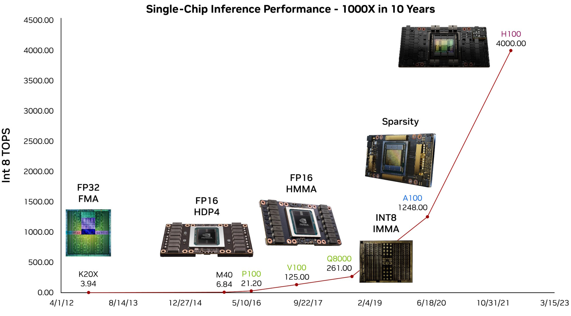
The increasing specialization of AI hardware has driven significant performance improvements in deep learning workloads. Figure 3 illustrates the trajectory of AI accelerator performance in NVIDIA GPUs, highlighting the transition from general-purpose floating-point execution units to highly optimized tensor processing cores.
Processing Elements
The highest level of execution unit organization integrates multiple tensor cores with local memory into processing elements (PEs). A processing element serves as a fundamental building block in many AI accelerators, combining different computational units to efficiently execute neural network operations. Each PE typically includes vector units for element-wise operations, tensor cores for matrix computation, special function units for non-linear transformations, and dedicated memory resources to optimize data locality and minimize data movement overhead.
Processing elements play an essential role in AI hardware by balancing computational density with memory access efficiency. Their design varies across different architectures to support diverse workloads and scalability requirements. Graphcore’s Intelligence Processing Unit (IPU) distributes computation across 1,472 tiles, each containing independent processing elements optimized for fine-grained parallelism (Graphcore 2020). Cerebras extends this approach in the CS-2 system, integrating 850,000 processing elements across a wafer-scale device to accelerate sparse computations. Tesla’s D1 processor arranges processing elements with substantial local memory, optimizing throughput and latency for real-time autonomous vehicle workloads (Quinnell 2024).
Graphcore. 2020. “The Colossus MK2 IPU Processor.” Graphcore Technical Paper.
Quinnell, Eric. 2024. “Tesla Transport Protocol over Ethernet (TTPoE): A New Lossy, Exa-Scale Fabric for the Dojo AI Supercomputer.” In 2024 IEEE Hot Chips 36 Symposium (HCS), 1–23. IEEE. https://doi.org/10.1109/hcs61935.2024.10664947.
Processing elements provide the structural foundation for large-scale AI acceleration. Their efficiency depends not only on computational capability but also on interconnect strategies and memory hierarchy design. The next sections explore how these architectural choices impact performance across different AI workloads.
Tensor processing units have enabled substantial efficiency gains in AI workloads by using hardware-accelerated matrix computation. Their role continues to evolve as architectures incorporate support for advanced execution techniques, including structured sparsity and workload-specific optimizations. The effectiveness of these units, however, depends not only on their computational capabilities but also on how they interact with memory hierarchies and data movement mechanisms, which are examined in subsequent sections.
Systolic Arrays
While tensor cores package matrix operations into structured computational units, systolic arrays provide an alternative approach optimized for continuous data flow and operand reuse. The fundamental motivation for systolic architectures stems from the energy efficiency constraints discussed earlier—minimizing the impact of memory access penalties through architectural design. A systolic array arranges processing elements in a grid pattern, where data flows rhythmically between neighboring units in a synchronized manner, enabling each operand to participate in multiple computations as it propagates through the array. This structured movement minimizes external memory accesses by maximizing local data reuse—a single weight value can contribute to dozens of operations as it moves through the processing elements, fundamentally transforming the energy profile from memory-bound to compute-efficient execution.
The concept of systolic arrays was first introduced by Kung and Leiserson24, who formalized their use in parallel computing architectures for efficient matrix operations (Kung 1982). Unlike general-purpose execution units, systolic arrays exploit spatial and temporal locality by reusing operands as they propagate through the grid. Google’s TPU exemplifies this architectural approach. In the TPUv4, a \(128\times128\) systolic array of multiply-accumulate units processes matrix operations by streaming data through the array in a pipelined manner, as shown in Figure 4.
24 Systolic Array Renaissance: H.T. Kung and Charles Leiserson introduced systolic arrays at CMU in 1979 for VLSI signal processing, but the concept languished for decades due to programming complexity. Google’s 2016 TPU resurrection proved these “heartbeat” architectures could deliver massive efficiency gains for neural networks—the TPUv1’s \(256\times 256\) systolic array achieved 92 TOPS for 8-bit integer operations while consuming just 40 watts, making systolic arrays the dominant AI architecture today.
Kung. 1982. “Why Systolic Architectures?” Computer 15 (1): 37–46. https://doi.org/10.1109/mc.1982.1653825.
The systolic array architecture achieves computational efficiency through synchronized data movement across a structured grid of processing elements. Systolic arrays organize computation around four fundamental components:
- Control Unit: Coordinates timing and data distribution across the array, maintaining synchronized operation throughout the computational grid
- Data Streams: Input matrices propagate through coordinated pathways—matrix A elements traverse horizontally while matrix B elements flow vertically through the processing grid
- Processing Element Grid: Individual processing elements execute multiply-accumulate operations on streaming data, generating partial results that accumulate toward the final computation
- Output Collection: Results aggregate at designated output boundaries where accumulated partial sums form complete matrix elements
The synchronized data flow ensures that matrix element A[i,k] encounters corresponding B[k,j] elements at precise temporal intervals, executing the multiply-accumulate operations required for matrix multiplication C[i,j] = Σ A[i,k] × B[k,j]. This systematic reuse of operands across multiple processing elements substantially reduces memory bandwidth requirements by eliminating redundant data fetches from external memory subsystems.
Consider the multiplication of 2×2 matrices A and B within a systolic array. During the first computational cycle, element A[0,0]=2 propagates horizontally while B[0,0]=1 moves vertically, converging at processing element PE(0,0) to execute the multiplication 2×1=2. In the subsequent cycle, the same A[0,0]=2 advances to PE(0,1) where it encounters B[0,1]=3, computing 2×3=6. Concurrently, A[0,1]=4 enters PE(0,0) to engage with the next B matrix element. This coordinated data movement enables systematic operand reuse across multiple computational operations, eliminating redundant memory accesses and exemplifying the fundamental efficiency principle underlying systolic array architectures.

Each processing element in the array performs a multiply-accumulate operation in every cycle:
- Receives an input activation from above
- Receives a weight value from the left
- Multiplies these values and adds to its running sum
- Passes the input activation downward and the weight value rightward to neighboring elements
This structured computation model minimizes data movement between global memory and processing elements, improving both efficiency and scalability. As systolic arrays operate in a streaming fashion, they are particularly effective for high-throughput workloads such as deep learning training and inference.
While the diagram in Figure 4 illustrates one common systolic array implementation, systolic architectures vary significantly across different accelerator designs. Training-focused architectures like Google’s TPU employ large arrays optimized for high computational throughput, while inference-oriented designs found in edge devices prioritize energy efficiency with smaller configurations.
The fundamental principle remains consistent: data flows systematically through processing elements, with inputs moving horizontally and vertically to compute partial sums in a synchronized fashion. However, as detailed in Section 1.4.1, practical effectiveness is ultimately constrained by memory bandwidth bottlenecks.
A 128×128 systolic array capable of 16,384 operations per cycle requires continuous data feed to maintain utilization—each cycle demands fresh input activations and weight parameters that must traverse from off-chip memory through on-chip buffers to the array edges. The TPU’s 1,200 GB/s on-chip bandwidth enables high utilization, but even this substantial bandwidth becomes limiting when processing large transformer models where memory requirements exceed on-chip capacity.
Recall from Chapter 10: Model Optimizations that quantization reduces model memory footprint by converting FP32 weights to INT8 representations—this optimization directly addresses the memory bandwidth constraints identified here. Converting 32-bit floating-point weights to 8-bit integers reduces memory traffic by 4×, transforming bandwidth-bound operations into compute-bound workloads where systolic arrays can achieve higher utilization. Similarly, structured pruning removes entire rows or columns of weight matrices, reducing both the data volume that must traverse memory hierarchies and the computation required. These algorithmic optimizations prove valuable precisely because they target the memory bottleneck that limits accelerator performance in practice.
Numerics in AI Acceleration
The efficiency of AI accelerators is not determined by computational power alone but also by the precision of numerical representations. The choice of numerical format shapes the balance between accuracy, throughput, and energy consumption, influencing how different execution units, such as SIMD and SIMT units, tensor cores, and systolic arrays, are designed and deployed.
Precision Trade-offs
Numerical precision represents a critical design parameter in modern AI accelerators. While higher precision formats provide mathematical stability and accuracy, they come with substantial costs in terms of power consumption, memory bandwidth, and computational throughput. Finding the optimal precision point has become a central challenge in AI hardware architecture.
Early deep learning models primarily relied on single-precision floating point (FP32) for both training and inference. While FP32 offers sufficient dynamic range and precision for stable learning, it imposes high computational and memory costs, limiting efficiency, especially as model sizes increase. Over time, hardware architectures evolved to support lower precision formats such as half-precision floating point (FP16) and bfloat16 (BF16), which reduce memory usage and increase computational throughput while maintaining sufficient accuracy for deep learning tasks. More recently, integer formats (INT8, INT4) have gained prominence in inference workloads, where small numerical representations significantly improve energy efficiency without compromising model accuracy beyond acceptable limits.
The transition from high-precision to lower-precision formats is deeply integrated into hardware execution models. As detailed in Section 1.3.4.2, SIMD and SIMT units provide flexible support for multiple precisions. Tensor cores (Section 1.3.4.3) accelerate computation using reduced-precision arithmetic, while systolic arrays (Section 1.3.4.5) optimize performance by minimizing memory bandwidth constraints through low-precision formats that maximize operand reuse.
Despite the advantages of reduced precision, deep learning models cannot always rely solely on low-bit representations. To address this challenge, modern AI accelerators implement mixed-precision computing, where different numerical formats are used at different stages of execution. These precision choices have important implications for model fairness and reliability. For example, matrix multiplications may be performed in FP16 or BF16, while accumulations are maintained in FP32 to prevent precision loss. Similarly, inference engines leverage INT8 arithmetic while preserving key activations in higher precision when necessary.
Mixed-Precision Computing
Modern AI accelerators increasingly support mixed-precision execution, allowing different numerical formats to be used at various stages of computation. Training workloads often leverage FP16 or BF16 for matrix multiplications, while maintaining FP32 accumulations to preserve precision. Inference workloads, by contrast, optimize for INT8 or even INT4, achieving high efficiency while retaining acceptable accuracy.
This shift toward precision diversity is evident in the evolution of AI hardware. Early architectures such as NVIDIA Volta provided limited support for lower precision beyond FP16, whereas later architectures, including Turing and Ampere, expanded the range of supported formats. Ampere GPUs introduced TF32 as a hybrid between FP32 and FP16, alongside broader support for BF16, INT8, and INT4. Table 5 illustrates this trend.
| Architecture | Year | Supported Tensor Core Precisions | Supported CUDA Core Precisions |
|---|---|---|---|
| Volta | 2017 | FP16 | FP64, FP32, FP16 |
| Turing | 2018 | FP16, INT8 | FP64, FP32, FP16, INT8 |
| Ampere | 2020 | FP64, TF32, bfloat16, FP16, INT8, INT4 | FP64, FP32, FP16, bfloat16, INT8 |
Table 5 highlights how newer architectures incorporate a growing diversity of numerical formats, reflecting the need for greater flexibility across different AI workloads. This trend suggests that future AI accelerators will continue expanding support for adaptive precision, optimizing both computational efficiency and model accuracy.
The precision format used in hardware design has far-reaching implications. By adopting lower-precision formats, the data transferred between execution units and memory is reduced, leading to decreased memory bandwidth requirements and storage. Tensor cores and systolic arrays can process more lower-precision elements in parallel, thereby increasing the effective throughput in terms of FLOPs. Energy efficiency is also improved, as integer-based computations (e.g., INT8) require lower power compared to floating-point arithmetic—a clear advantage for inference workloads.
As AI models continue to scale in size, accelerator architectures are evolving to support more efficient numerical formats. Future designs are expected to incorporate adaptive precision techniques, dynamically adjusting computation precision based on workload characteristics. This evolution promises further optimization of deep learning performance while striking an optimal balance between accuracy and energy efficiency.
Architectural Integration
The organization of computational primitives into execution units determines the efficiency of AI accelerators. While SIMD, tensor cores, and systolic arrays serve as fundamental building blocks, their integration into full-chip architectures varies significantly across different AI processors. The choice of execution units, their numerical precision support, and their connectivity impact how effectively hardware can scale for deep learning workloads.
Modern AI processors exhibit a range of design trade-offs based on their intended applications. Some architectures, such as NVIDIA’s A100, integrate large numbers of tensor cores optimized for FP16-based training, while Google’s TPUv4 prioritizes high-throughput BF16 matrix multiplications. Inference-focused processors, such as Intel’s Sapphire Rapids, incorporate INT8-optimized tensor cores to maximize efficiency. The Apple M1, designed for mobile workloads, employs smaller processing elements optimized for low-power FP16 execution. These design choices reflect the growing flexibility in numerical precision and execution unit organization, as discussed in the previous section.
Table 6 summarizes the execution unit configurations across contemporary AI processors.
| Processor | SIMD Width | Tensor Core Size | Processing Elements | Primary Workloads |
|---|---|---|---|---|
| NVIDIA A100 | 1024-bit | \(4\times4\times4\) FP16 | 108 SMs | Training, HPC |
| Google TPUv4 | 128-wide | \(128\times128\) BF16 | 2 cores/chip | Training |
| Intel Sapphire | 512-bit AVX | \(32\times32\) INT8/BF16 | 56 cores | Inference |
| Apple M1 | 128-bit NEON | \(16\times16\) FP16 | 8 NPU cores | Mobile inference |
Table 6 highlights how execution unit configurations vary across architectures to optimize for different deep learning workloads. Training accelerators prioritize high-throughput floating-point tensor operations, whereas inference processors focus on low-precision integer execution for efficiency. Meanwhile, mobile accelerators balance precision and power efficiency to meet real-time constraints.
Cost-Performance Analysis
While architectural specifications define computational potential, practical deployment decisions require understanding cost-performance trade-offs across different accelerator options. However, raw computational metrics alone provide an incomplete picture—the fundamental constraint in modern AI acceleration is not compute capacity but data movement efficiency.
The energy differential established earlier—where memory access costs dominate computation—drives the entire specialized hardware revolution. This disparity explains why GPUs with high memory bandwidth achieve 40-60% utilization, while TPUs with systolic arrays achieve 85% utilization by minimizing data movement.
Table 7 provides concrete cost-performance data for representative accelerators, but the economic analysis must account for utilization efficiency and energy consumption patterns that determine real-world performance.
| Accelerator | List Price (USD) | Peak FLOPS (FP16) | Memory Bandwidth | Price/Performance |
|---|---|---|---|---|
| NVIDIA V100 | ~$9,000 (2017-19) | 125 TFLOPS | 900 GB/s | $72/TFLOP |
| NVIDIA A100 | $15,000 | 312 TFLOPS (FP16) | 1,935 GB/s | $48/TFLOP |
| NVIDIA H100 | $25,000-30,000 | 756 TFLOPS (TF32) | 3,350 GB/s | $33/TFLOP |
| Google TPUv4 | ~$8,000* | 275 TFLOPS (BF16) | 1,200 GB/s | $29/TFLOP |
| Intel H100 | $12,000 | 200 TFLOPS (INT8) | 800 GB/s | $60/TFLOP |
A startup training large language models faces the choice between 8 V100s ($72K) providing 1,000 TFLOPS or 4 A100s ($60K) delivering 1,248 TFLOPS. However, performance analysis reveals the true performance story—transformer training with its arithmetic intensity of 0.5-2 FLOPS/byte makes both configurations memory-bandwidth bound rather than compute-bound. The A100’s 1,935 GB/s bandwidth delivers 2.15× higher sustainable performance than V100’s 900 GB/s, making the effective performance gain 115% rather than the 25% suggested by peak FLOPS. When combined with 17% lower hardware cost and 30% better energy efficiency (400 W vs 300 W per effective TFLOP), the A100 configuration provides compelling economic advantages that compound over multi-year deployments.
These cost dynamics explain the rapid adoption of newer accelerators despite higher unit prices. The H100’s $33/TFLOP represents a 54% improvement over V100’s $72/TFLOP, but more importantly, its 3,350 GB/s bandwidth enables 3.7× higher memory throughput per dollar—the metric that determines real-world transformer performance. Cloud deployment further complicates the analysis, as providers typically charge $2-4/hour for high-end accelerators, making the break-even point between purchase and rental highly dependent on utilization patterns and energy costs that can account for 60-70% of total operational expenses over a three-year lifecycle.
Framework selection significantly impacts these economic decisions—detailed hardware-framework optimization strategies are covered in Chapter 7: AI Frameworks, while performance evaluation methodologies are discussed in Chapter 12: Benchmarking AI.
While execution units define the compute potential of an accelerator, their effectiveness is fundamentally constrained by data movement and memory hierarchy. Achieving high utilization of compute resources requires efficient memory systems that minimize data transfer overhead and optimize locality. Understanding these constraints reveals why memory architecture becomes as critical as computational design in AI acceleration.
AI Memory Systems
The execution units examined in previous sections—SIMD units, tensor cores, and systolic arrays—provide impressive computational throughput: modern accelerators achieve 100 to 1000 TFLOPS for neural network operations. Yet these theoretical capabilities remain unrealized in practice when memory subsystems cannot supply data at sufficient rates. This fundamental constraint, termed the AI memory wall, represents the dominant bottleneck in real-world accelerator performance.
Unlike conventional workloads, ML models require frequent access to large volumes of parameters, activations, and intermediate results, leading to substantial memory bandwidth demands—a challenge that intersects with the data management strategies covered in Chapter 6: Data Engineering. Modern AI hardware addresses these challenges through advanced memory hierarchies, efficient data movement techniques, and compression strategies that promote efficient execution and improved AI acceleration.
This section examines memory system design through four interconnected perspectives. First, we quantify the growing disparity between computational throughput and memory bandwidth, revealing why the AI memory wall represents the dominant performance constraint in modern accelerators. Second, we explore how memory hierarchies balance competing demands for speed, capacity, and energy efficiency through carefully structured tiers from on-chip SRAM to off-chip DRAM. Third, we analyze communication patterns between host systems and accelerators, exposing transfer bottlenecks that limit end-to-end performance. Finally, we examine how different neural network architectures—multilayer perceptrons, convolutional networks, and transformers—create distinct memory pressure patterns that inform hardware design decisions and optimization strategies.
Understanding the AI Memory Wall
The AI memory wall represents the fundamental bottleneck constraining modern accelerator performance—the growing disparity between computational throughput and memory bandwidth that prevents accelerators from achieving their theoretical capabilities. While compute units can execute millions of operations per second through specialized primitives like vector operations and matrix multiplications, they depend entirely on memory systems to supply the continuous stream of weights, activations, and intermediate results these operations require.
Quantifying the Compute-Memory Performance Gap
The severity of this constraint becomes apparent when examining scaling trends. Over the past 20 years, peak computational capabilities have scaled at 3.0× every two years, while DRAM bandwidth has grown at only 1.6× during the same period (Gholami et al. 2024). This divergence creates an exponentially widening gap where accelerators possess massive computational power but cannot access data quickly enough to utilize it. Modern hardware exemplifies this imbalance: an NVIDIA H100 delivers 989 TFLOPS but only 3.35 TB/s memory bandwidth (Choquette 2023), requiring 295 operations per byte to achieve full utilization—far exceeding the 1-10 operations per byte typical in neural networks.
Gholami, Amir, Zhewei Yao, Sehoon Kim, Coleman Hooper, Michael W. Mahoney, and Kurt Keutzer. 2024. “AI and Memory Wall.” IEEE Micro 44 (3): 33–39. https://doi.org/10.1109/mm.2024.3373763.
The memory wall manifests through three critical constraints. First, the energy disparity—accessing DRAM consumes 640 pJ compared to 3.7 pJ for computation (Horowitz 2014), creating a 173× energy penalty that often limits performance due to power budgets rather than computational capacity. Second, the bandwidth limitation—even TB/s memory systems cannot feed thousands of parallel compute units continuously, forcing 50-70% idle time in typical workloads. Third, the latency hierarchy—off-chip memory access requires hundreds of cycles, creating pipeline stalls that cascade through parallel execution units.
As illustrated in Figure 5, this “AI Memory Wall” continues to widen, making memory bandwidth rather than compute the primary constraint in AI acceleration.
Beyond performance limitations, memory access imposes a significant energy cost. Fetching data from off-chip DRAM consumes far more energy than performing arithmetic operations (Horowitz 2014). This inefficiency is particularly evident in machine learning models, where large parameter sizes, frequent memory accesses, and non-uniform data movement patterns exacerbate memory bottlenecks. The energy differential drives architectural decisions—Google’s TPU achieves 30-83\(\times\) better energy efficiency than contemporary GPUs by minimizing data movement through systolic arrays and large on-chip memory. These design choices demonstrate that energy constraints, not computational limits, often determine practical deployment feasibility.
Horowitz, Mark. 2014. “1.1 Computing’s Energy Problem (and What We Can Do about It).” In 2014 IEEE International Solid-State Circuits Conference Digest of Technical Papers (ISSCC). IEEE. https://doi.org/10.1109/isscc.2014.6757323.
Memory Access Patterns in ML Workloads
Machine learning workloads place substantial demands on memory systems due to the large volume of data involved in computation. Unlike traditional compute-bound applications, where performance is often dictated by the speed of arithmetic operations, ML workloads are characterized by high data movement requirements. The efficiency of an accelerator is not solely determined by its computational throughput but also by its ability to continuously supply data to processing units without introducing stalls or delays.
A neural network processes multiple types of data throughout its execution, each with distinct memory access patterns:
- Model parameters (weights and biases): Machine learning models, particularly those used in large-scale applications such as natural language processing and computer vision, often contain millions to billions of parameters. Storing and accessing these weights efficiently is essential for maintaining throughput.
- Intermediate activations: During both training and inference, each layer produces intermediate results that must be temporarily stored and retrieved for subsequent operations. These activations can contribute significantly to memory overhead, particularly in deep architectures.
- Gradients (during training): Backpropagation requires storing and accessing gradients for every parameter, further increasing the volume of data movement between compute units and memory.
As models increase in size and complexity, improvements in memory capacity and bandwidth become essential. Although specialized compute units accelerate operations like matrix multiplications, their overall performance depends on the continuous, efficient delivery of data to the processing elements. In large-scale applications, such as natural language processing and computer vision, models often incorporate millions to billions of parameters (Brown et al. 2020). Consequently, achieving high performance necessitates minimizing delays and stalls caused by inefficient data movement between memory and compute units (Narayanan et al. 2021; Xingyu 2019).
Xingyu, Huang et al. 2019. “Addressing the Memory Bottleneck in AI Accelerators.” IEEE Micro.
One way to quantify this challenge is by comparing the data transfer time with the time required for computations. Specifically, we define the memory transfer time as \[ T_{\text{mem}} = \frac{M_{\text{total}}}{B_{\text{mem}}}, \] where \(M_{\text{total}}\) is the total data volume and \(B_{\text{mem}}\) is the available memory bandwidth. In contrast, the compute time is given by \[ T_{\text{compute}} = \frac{\text{FLOPs}}{P_{\text{peak}}}, \] with the number of floating-point operations (FLOPs) divided by the peak hardware throughput, \(P_{\text{peak}}\). When \(T_{\text{mem}} > T_{\text{compute}}\), the system becomes memory-bound, meaning that the processing elements spend more time waiting for data than performing computations. This imbalance demonstrates the need for memory-optimized architectures and efficient data movement strategies to sustain high performance.
Figure 6 demonstrates the emerging challenge between model growth and hardware memory capabilities, illustrating the “AI Memory Wall.” The figure tracks AI model sizes (red dots) and hardware memory bandwidth (blue dots) over time on a log scale. Model parameters have grown exponentially, from AlexNet’s ~62.3M parameters in 2012 to Gemini 1’s trillion-scale parameters in 2023, as shown by the steeper red trend line. In contrast, hardware memory bandwidth, represented by successive generations of NVIDIA GPUs (~100-200 GB/s) and Google TPUs (~2-3 TB/s), has increased more gradually (blue trend line). The expanding shaded region between these trends corresponds to the “AI Memory Wall,” which will be an architectural challenge where model scaling outpaces available memory bandwidth. This growing disparity necessitates increasingly sophisticated memory management and model optimization techniques to maintain computational efficiency.
Irregular Memory Access
Unlike traditional computing workloads, where memory access follows well-structured and predictable patterns, machine learning models often exhibit irregular memory access behaviors that make efficient data retrieval a challenge. These irregularities arise due to the nature of ML computations, where memory access patterns are influenced by factors such as batch size, layer type, and sparsity. As a result, standard caching mechanisms and memory hierarchies often struggle to optimize performance, leading to increased memory latency and inefficient bandwidth utilization.
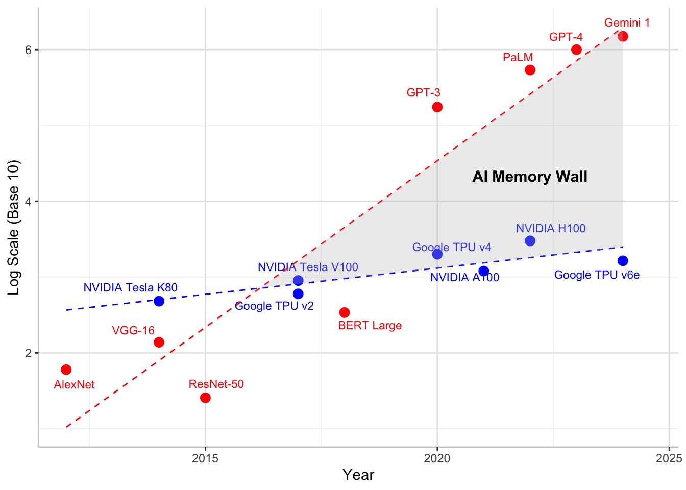
To better understand how ML workloads differ from traditional computing workloads, it is useful to compare their respective memory access patterns (Table 8). Traditional workloads, such as scientific computing, general-purpose CPU applications, and database processing, typically exhibit well-defined memory access characteristics that benefit from standard caching and prefetching techniques. ML workloads, on the other hand, introduce highly dynamic access patterns that challenge conventional memory optimization strategies.
One key source of irregularity in ML workloads stems from batch size and execution order. The way input data is processed in batches directly affects memory reuse, creating a complex optimization challenge. Small batch sizes decrease the likelihood of reusing cached activations and weights, resulting in frequent memory fetches from slower, off-chip memory. Larger batch sizes can improve reuse and amortize memory access costs, but simultaneously place higher demands on available memory bandwidth, potentially creating congestion at different memory hierarchy levels. This delicate balance requires careful consideration of model architecture and available hardware resources.
| Feature | Traditional Computing Workloads | Machine Learning Workloads |
|---|---|---|
| Memory Access Pattern | Regular and predictable (e.g., sequential reads, structured patterns) | Irregular and dynamic (e.g., sparsity, attention mechanisms) |
| Cache Locality | High temporal and spatial locality | Often low locality, especially in large models |
| Data Reuse | Structured loops with frequent data reuse | Sparse and dynamic reuse depending on layer type |
| Data Dependencies | Well-defined dependencies allow efficient prefetching | Variable dependencies based on network structure |
| Workload Example | Scientific computing (e.g., matrix factorizations, physics simulations) | Neural networks (e.g., CNNs, Transformers, sparse models) |
| Memory Bottleneck | DRAM latency, cache misses | Off-chip bandwidth constraints, memory fragmentation |
| Impact on Energy Consumption | Moderate, driven by FLOP-heavy execution | High, dominated by data movement costs |
Different neural network layers interact with memory in distinct ways beyond batch size considerations. Convolutional layers benefit from spatial locality, as neighboring pixels in an image are processed together, enabling efficient caching of small weight kernels. Conversely, fully connected layers require frequent access to large weight matrices, often leading to more randomized memory access patterns that poorly align with standard caching policies. Transformers introduce additional complexity, as attention mechanisms demand accessing large key-value pairs stored across varied memory locations. The dynamic nature of sequence length and attention span renders traditional prefetching strategies ineffective, resulting in unpredictable memory latencies.
Another significant factor contributing to irregular memory access is sparsity25 in neural networks. Many modern ML models employ techniques such as weight pruning, activation sparsity, and structured sparsity to reduce computational overhead. However, these optimizations often lead to non-uniform memory access, as sparse representations necessitate fetching scattered elements rather than sequential blocks, making hardware caching less effective. Models that incorporate dynamic computation paths, such as Mixture of Experts and Adaptive Computation Time, introduce highly non-deterministic memory access patterns, where the active neurons or model components can vary with each inference step. This variability challenges efficient prefetching and caching strategies.
25 Sparsity in Neural Networks: The property that most weights or activations in a neural network are zero or near-zero, enabling computational and memory optimizations. Natural sparsity occurs when ReLU activations zero out 50-90% of values, while artificial sparsity results from pruning techniques that remove 90-99% of weights with minimal accuracy loss. Sparse networks can be 10-100\(\times\) smaller and faster, but require specialized hardware support (like NVIDIA’s 2:4 sparsity in A100) or software optimization to realize benefits, as standard dense hardware performs zero multiplications inefficiently.
These irregularities have significant consequences. ML workloads often experience reduced cache efficiency, as activations and weights may not be accessed in predictable sequences. This leads to increased reliance on off-chip memory traffic, which slows down execution and consumes more energy. Irregular access patterns contribute to memory fragmentation, where the way data is allocated and retrieved results in inefficient utilization of available memory resources. The combined effect is that ML accelerators frequently encounter memory bottlenecks that limit their ability to fully utilize available compute power.
Memory Hierarchy
To address the memory challenges in ML acceleration, hardware designers implement sophisticated memory hierarchies that balance speed, capacity, and energy efficiency. Understanding this hierarchy is essential before examining how different ML architectures utilize memory resources. Unlike general-purpose computing, where memory access patterns are often unpredictable, ML workloads exhibit structured reuse patterns that can be optimized through careful organization of data across multiple memory levels.
At the highest level, large-capacity but slow storage devices provide long-term model storage. At the lowest level, high-speed registers and caches ensure that compute units can access operands with minimal latency. Between these extremes, intermediate memory levels, such as scratchpad memory, high-bandwidth memory, and off-chip DRAM, offer trade-offs between performance and capacity.
Table 9 summarizes the key characteristics of different memory levels in modern AI accelerators. Each level in the hierarchy has distinct latency, bandwidth, and capacity properties, which directly influence how neural network data, such as weights, activations, and intermediate results, should be allocated.
| Memory Level | Approx. Latency | Bandwidth | Capacity | Example Use in Deep Learning |
|---|---|---|---|---|
| Registers | ~1 cycle | Highest | Few values | Storing operands for immediate computation |
| L1/L2 Cache (SRAM) | ~1-10 ns | High | KBs-MBs | Caching frequently accessed activations and small weight blocks |
| Scratchpad Memory | ~5-20 ns | High | MBs | Software-managed storage for intermediate computations |
| High-Bandwidth Memory (HBM) | ~100 ns | Very High | GBs | Storing large model parameters and activations for high-speed access |
| Off-Chip DRAM (DDR, GDDR, LPDDR) | ~50-150 ns | Moderate | GBs-TBs | Storing entire model weights that do not fit on-chip |
| Flash Storage (SSD/NVMe) | ~100 µs - 1 ms | Low | TBs | Storing pre-trained models and checkpoints for later loading |
On-Chip Memory
Each level of the memory hierarchy serves a distinct role in AI acceleration, with different trade-offs in speed, capacity, and accessibility. Registers, located within compute cores, provide the fastest access but can only store a few operands at a time. These are best utilized for immediate computations, where the operands needed for an operation can be loaded and consumed within a few cycles. However, because register storage is so limited, frequent memory accesses are required to fetch new operands and store intermediate results.
To reduce the need for constant data movement between registers and external memory, small but fast caches serve as an intermediary buffer. These caches store recently accessed activations, weights, and intermediate values, ensuring that frequently used data remains available with minimal delay. However, the size of caches is limited, making them insufficient for storing full feature maps or large weight tensors in machine learning models. As a result, only the most frequently used portions of a model’s parameters or activations can reside here at any given time.
For larger working datasets, many AI accelerators include scratchpad memory, which offers more storage than caches but with a crucial difference: it allows explicit software control over what data is stored and when it is evicted. Unlike caches, which rely on hardware-based eviction policies, scratchpad memory enables machine learning workloads to retain key values such as activations and filter weights for multiple layers of computation. This capability is particularly useful in models like convolutional neural networks, where the same input feature maps and filter weights are reused across multiple operations. By keeping this data in scratchpad memory rather than reloading it from external memory, accelerators can significantly reduce unnecessary memory transfers and improve overall efficiency (Chen, Emer, and Sze 2017).
Off-Chip Memory
Beyond on-chip memory, high-bandwidth memory provides rapid access to larger model parameters and activations that do not fit within caches or scratchpad buffers. HBM achieves its high performance by stacking multiple memory dies and using wide memory interfaces, allowing it to transfer large amounts of data with minimal latency compared to traditional DRAM. Because of its high bandwidth and lower latency, HBM is often used to store entire layers of machine learning models that must be accessed quickly during execution. However, its cost and power consumption limit its use primarily to high-performance AI accelerators, making it less common in power-constrained environments such as edge devices.
When a machine learning model exceeds the capacity of on-chip memory and HBM, it must rely on off-chip DRAM, such as DDR, GDDR, or LPDDR. While DRAM offers significantly greater storage capacity, its access latency is higher, meaning that frequent retrievals from DRAM can introduce execution bottlenecks. To make effective use of DRAM, models must be structured so that only the necessary portions of weights and activations are retrieved at any given time, minimizing the impact of long memory fetch times.
At the highest level of the hierarchy, flash storage and solid-state drives (SSDs) store large pre-trained models, datasets, and checkpointed weights. These storage devices offer large capacities but are too slow for real-time execution, requiring models to be loaded into faster memory tiers before computation begins. For instance, in training scenarios, checkpointed models stored in SSDs must be loaded into DRAM or HBM before resuming computation, as direct execution from SSDs would be too slow to maintain efficient accelerator utilization (Narayanan et al. 2021).
The memory hierarchy balances competing objectives of speed, capacity, and energy efficiency. However, moving data through multiple memory levels introduces bottlenecks that limit accelerator performance. Data transfers between memory levels incur latency costs, particularly for off-chip accesses. Limited bandwidth restricts data flow between memory tiers. Memory capacity constraints force constant data movement as models exceed local storage. These constraints make memory bandwidth the fundamental determinant of real-world accelerator performance.
Memory Bandwidth and Architectural Trade-offs
Building on the memory wall analysis established in Section 1.4.1, this section quantifies how specific bandwidth characteristics impact system performance across different deployment scenarios.
Modern accelerators exhibit distinct bandwidth-capacity trade-offs: NVIDIA H100 GPUs provide 3.35 TB/s HBM3 bandwidth with 80 GB capacity, optimizing for flexibility across diverse workloads. Google’s TPUv4 delivers 1.2 TB/s bandwidth with 128 MB on-chip memory, prioritizing energy efficiency for tensor operations. This 3:1 bandwidth advantage enables H100 to handle memory-intensive models like large language models, while TPU’s lower bandwidth suffices for compute-intensive inference due to superior data reuse.
Different neural network operations achieve varying bandwidth utilization: transformer attention mechanisms achieve only 20-40% of peak memory bandwidth due to irregular access patterns, convolutional layers achieve 60-85% through predictable spatial access patterns, and fully connected layers approach 90% when batch sizes exceed 128.
As established earlier, on-chip memory access consumes 5-10 pJ per access, while external DRAM requires 640 pJ per access—a 65-125\(\times\) energy penalty. AI accelerators minimize DRAM access through three key strategies: weight stationarity (keeping model parameters in on-chip memory), input stationarity (buffering input activations locally), and output stationarity (accumulating partial sums on-chip).
Memory bandwidth scaling follows different trajectories across accelerator designs:
- GPU scaling: Bandwidth increases linearly with memory channels, from 900 GB/s (A100) to 3,350 GB/s (H100), enabling larger model support
- TPU scaling: Bandwidth optimization through systolic array design achieves 900 GB/s with 35% lower power than GPU alternatives
- Mobile accelerator scaling: Apple’s M3 Neural Engine achieves 400 GB/s unified memory bandwidth while consuming <5 W through aggressive voltage scaling
HBM memory costs $8-15 per GB compared to $0.05 per GB for DDR5, creating 160-300\(\times\) cost differences. High-bandwidth accelerators require 40-80 GB HBM for competitive performance, adding $320-1,200 to manufacturing costs. Edge accelerators sacrifice bandwidth (50-200 GB/s) to achieve sub-$100 cost targets while maintaining sufficient performance for inference workloads.
These bandwidth characteristics directly influence deployment decisions: cloud training prioritizes raw bandwidth for maximum model capacity, edge inference optimizes bandwidth efficiency for energy constraints, and mobile deployment balances bandwidth with cost limitations. While these hardware-specific optimizations are fundamental, the integrated system-level efficiency approaches that combine hardware acceleration with software optimization techniques are comprehensively covered in Chapter 9: Efficient AI. The deployment of these optimizations across different system contexts—from mobile devices in Chapter 2: ML Systems to production workflows in Chapter 13: ML Operations—determines their real-world impact.
Host-Accelerator Communication
Machine learning accelerators, such as GPUs and TPUs, achieve high computational throughput through parallel execution. However, their efficiency is fundamentally constrained by data movement between the host (CPU) and accelerator memory. Unlike general-purpose workloads that operate entirely within a CPU’s memory subsystem, AI workloads require frequent data transfers between CPU main memory and the accelerator, introducing latency, consuming bandwidth, and affecting overall performance.
Host-accelerator data movement follows a structured sequence, as illustrated in Figure 7. Before computation begins, data is copied from CPU memory to the accelerator’s memory. The CPU then issues execution instructions, and the accelerator processes the data in parallel. Once computation completes, the results are stored in accelerator memory and transferred back to the CPU. Each step introduces potential inefficiencies that must be managed to optimize performance.

The key challenges in host-accelerator data movement include latency, bandwidth constraints, and synchronization overheads. Optimizing data transfers through efficient memory management and interconnect technologies is essential for maximizing accelerator utilization.
Data Transfer Patterns
The efficiency of ML accelerators depends not only on their computational power but also on the continuous supply of data. Even high-performance GPUs and TPUs remain underutilized if data transfers are inefficient. Host and accelerator memory exist as separate domains, requiring explicit transfers over interconnects such as PCIe, NVLink, or proprietary links. Ineffective data movement can cause execution stalls, making transfer optimization critical.
Figure 7 illustrates this structured sequence. In step (1), data is copied from CPU memory to accelerator memory, as GPUs cannot directly access host memory at high speeds. A direct memory access (DMA)26 engine typically handles this transfer without consuming CPU cycles. In step (2), the CPU issues execution commands via APIs like CUDA, ROCm, or OpenCL. Step (3) involves parallel execution on the accelerator, where stalls can occur if data is not available when needed. Finally, in step (4), computed results are copied back to CPU memory for further processing.
26 Direct Memory Access (DMA): Hardware mechanism that enables devices to transfer data to/from memory without CPU intervention. First introduced in 1981 with IBM’s PC, DMA engines free the CPU to perform other tasks while data moves between system memory and accelerators. Modern GPUs contain multiple DMA engines achieving 32 GB/s (PCIe 4.0) to 900 GB/s (NVLink) transfer rates. This asynchronous capability is crucial for AI workloads where data movement can overlap with computation, improving overall system utilization.
Latency and bandwidth limitations significantly impact AI workloads. PCIe, with a peak bandwidth of 32 GB/s (PCIe 4.0), is much slower than an accelerator’s high-bandwidth memory, which can exceed 1 TB/s. Large data transfers exacerbate bottlenecks, particularly in deep learning tasks. Additionally, synchronization overheads arise when computation must wait for data transfers to complete. Efficient scheduling and overlapping transfers with execution are essential to mitigate these inefficiencies.
Data Transfer Mechanisms
The movement of data between the host (CPU) and the accelerator (GPU, TPU, or other AI hardware) depends on the interconnect technology that links the two processing units. The choice of interconnect determines the bandwidth available for transfers, the latency of communication, and the overall efficiency of host-accelerator execution. The most commonly used transfer mechanisms include PCIe (Peripheral Component Interconnect Express), NVLink, Direct Memory Access, and Unified Memory Architectures. Each of these plays a crucial role in optimizing the four-step data movement process illustrated in Figure 7.
PCIe Interface
Most accelerators communicate with the CPU via PCIe, the industry-standard interconnect for data movement. PCIe 4.0 provides up to 32 GB/s bandwidth, while PCIe 5.0 doubles this to 64 GB/s. However, this is still significantly lower than HBM bandwidth within accelerators, making PCIe a bottleneck for large AI workloads.
PCIe also introduces latency overheads due to its packet-based communication and memory-mapped I/O model. Frequent small transfers are inefficient, so batching data movement reduces overhead. Computation commands, issued over PCIe, further contribute to latency, requiring careful optimization of execution scheduling.
NVLink Interface
To address the bandwidth limitations of PCIe, NVIDIA developed NVLink, a proprietary high-speed interconnect that provides significantly higher bandwidth between GPUs and, in some configurations, between the CPU and GPU. Unlike PCIe, which operates as a shared bus, NVLink enables direct point-to-point communication between connected devices, reducing contention and improving efficiency for AI workloads.
For host-accelerator transfers, NVLink can be used in step (1) to transfer input data from main memory to GPU memory at speeds far exceeding PCIe, with bandwidths reaching up to 600 GB/s in NVLink 4.0. This significantly reduces the data movement bottleneck, allowing accelerators to access input data with lower latency. In multi-GPU configurations, NVLink also accelerates peer-to-peer transfers, allowing accelerators to exchange data without routing through main memory, thereby optimizing step (3) of the computation process.
Although NVLink offers substantial performance benefits, it is not universally available. Unlike PCIe, which is an industry standard across all accelerators, NVLink is specific to NVIDIA hardware, limiting its applicability to systems designed with NVLink-enabled GPUs.
DMA for Data Transfers
In conventional memory transfers, the CPU issues load/store instructions, consuming processing cycles. DMA offloads this task, enabling asynchronous data movement without CPU intervention.
During data transfers, the CPU initiates a DMA request, allowing data to be copied to accelerator memory in the background. Similarly, result transfers back to main memory occur without blocking execution. This enables overlapping computation with data movement, reducing idle time and improving accelerator utilization.
DMA is essential for enabling asynchronous data movement, which allows transfers to overlap with computation. Instead of waiting for transfers to complete before execution begins, AI workloads can stream data into the accelerator while earlier computations are still in progress, reducing idle time and improving accelerator utilization.
Unified Memory
While PCIe, NVLink, and DMA optimize explicit memory transfers, some AI workloads require a more flexible memory model that eliminates the need for manual data copying. Unified Memory provides an abstraction that allows both the host and accelerator to access a single, shared memory space, automatically handling data movement when needed.
With Unified Memory, data does not need to be explicitly copied between CPU and GPU memory before execution. Instead, when a computation requires a memory region that is currently located in host memory, the system automatically migrates it to the accelerator, handling step (1) transparently. Similarly, when computed results are accessed by the CPU, step (4) occurs automatically, eliminating the need for manual memory management.
Although Unified Memory simplifies programming, it introduces performance trade-offs. Since memory migrations occur on demand, they can lead to unpredictable latencies, particularly if large datasets need to be transferred frequently. Additionally, since Unified Memory is implemented through page migration techniques, small memory accesses can trigger excessive data movement, further reducing efficiency.
For AI workloads that require fine-grained memory control, explicit data transfers using PCIe, NVLink, and DMA often provide better performance. However, for applications where ease of development is more important than absolute speed, Unified Memory offers a convenient alternative.
Data Transfer Overheads
Host-accelerator data movement introduces overheads that impact AI workload execution. Unlike on-chip memory accesses, which occur at nanosecond latencies, host-accelerator transfers traverse system interconnects, adding latency, bandwidth constraints, and synchronization delays.
Interconnect latency affects transfer speed, with PCIe, the standard host-accelerator link, incurring significant overhead due to packet-based transactions and memory-mapped I/O. This makes frequent small transfers inefficient. Faster alternatives like NVLink reduce latency and improve bandwidth but are limited to specific hardware ecosystems.
Synchronization delays further contribute to inefficiencies. Synchronous transfers block execution until data movement completes, ensuring data consistency but introducing idle time. Asynchronous transfers allow computation and data movement to overlap, reducing stalls but requiring careful coordination to avoid execution mismatches.
These factors, including interconnect latency, bandwidth limitations, and synchronization overheads, determine AI workload efficiency. While optimization techniques mitigate these limitations, understanding these fundamental transfer mechanics is essential for improving performance.
Model Memory Pressure
Machine learning models impose varying memory access patterns that significantly influence accelerator performance. The way data is transferred between the host and accelerator, how frequently memory is accessed, and the efficiency of caching mechanisms all determine overall execution efficiency. While multilayer perceptrons (MLPs), convolutional neural networks (CNNs), and transformer networks each require large parameter sets, their distinct memory demands necessitate tailored optimization strategies for accelerators. Understanding these differences provides insight into why different hardware architectures exhibit varying levels of efficiency across workloads.
Multilayer Perceptrons
MLPs, also referred to as fully connected networks, are among the simplest neural architectures. Each layer consists of a dense matrix multiplication, requiring every neuron to interact with all neurons in the preceding layer. This results in high memory bandwidth demands, particularly for weights, as every input activation contributes to a large set of computations.
From a memory perspective, MLPs rely on large, dense weight matrices that frequently exceed on-chip memory capacity, necessitating off-chip memory accesses. Since accelerators cannot directly access host memory at high speed, data transfers must be explicitly managed via interconnects such as PCIe or NVLink. These transfers introduce latency and consume bandwidth, affecting execution efficiency.
Despite their bandwidth-heavy nature, MLPs exhibit regular and predictable memory access patterns, making them amenable to optimizations such as prefetching and streaming memory accesses. Dedicated AI accelerators mitigate transfer overhead by staging weight matrices in fast SRAM caches and overlapping data movement with computation through direct memory access engines, reducing execution stalls. These optimizations allow accelerators to sustain high throughput even when handling large parameter sets (Chen, Emer, and Sze 2017).
Convolutional Neural Networks
Convolutional Neural Networks (CNNs) are widely used in image processing and computer vision tasks. Unlike MLPs, which require dense matrix multiplications, CNNs process input feature maps using small filter kernels that slide across the image. This localized computation structure results in high spatial data reuse, where the same input pixels contribute to multiple convolutions.
CNN accelerators benefit from on-chip memory optimizations, as convolution filters exhibit extensive reuse, allowing weights to be stored in fast local SRAM instead of frequently accessing off-chip memory. However, activation maps require careful management due to their size. Since accessing main memory over interconnects like PCIe introduces latency and bandwidth bottlenecks, CNN accelerators employ tiling techniques to divide feature maps into smaller regions that fit within on-chip buffers. This minimizes costly external memory transfers, improving overall efficiency (Chen, Emer, and Sze 2017).
Chen, Yu-Hsin, Joel Emer, and Vivienne Sze. 2017. “Using Dataflow to Optimize Energy Efficiency of Deep Neural Network Accelerators.” IEEE Micro 37 (3): 12–21. https://doi.org/10.1109/mm.2017.54.
While CNN workloads are more memory-efficient than MLPs, managing intermediate activations remains a challenge. Accelerators use hierarchical caching strategies and DMA engines to optimize memory movement, ensuring that computations are not stalled by inefficient host-accelerator data transfers. These memory optimizations help CNN accelerators maintain high throughput by reducing reliance on off-chip memory bandwidth (Chen, Emer, and Sze 2017).
Transformer Networks
Transformers have become the dominant architecture for natural language processing and are increasingly used in other domains such as vision and speech recognition. Unlike CNNs, which rely on local computations, transformers perform global attention mechanisms, where each token in an input sequence can interact with all other tokens. This leads to irregular and bandwidth-intensive memory access patterns, as large key-value matrices must be fetched and updated frequently.
These models are particularly challenging for accelerators due to their massive parameter sizes, which often exceed on-chip memory capacity. As a result, frequent memory transfers between host and accelerator introduce substantial latency overheads, particularly when relying on interconnects such as PCIe. Unified Memory architectures can mitigate some of these issues by dynamically handling data movement, but they introduce additional latency due to unpredictable on-demand memory migrations. Because transformers are memory-bound rather than compute-bound, accelerators optimized for them rely on high-bandwidth memory, tensor tiling, and memory partitioning to sustain performance (Brown et al. 2020).
Brown, Tom B., Benjamin Mann, Nick Ryder, Melanie Subbiah, Jared Kaplan, Prafulla Dhariwal, Arvind Neelakantan, et al. 2020. “Language Models Are Few-Shot Learners.” NeurIPS, May. http://arxiv.org/abs/2005.14165v4.
Narayanan, Deepak, Mohammad Shoeybi, Jared Casper, Patrick LeGresley, Mostofa Patwary, Vijay Anand Korthikanti, Dmitri Vainbrand, et al. 2021. “Efficient Large-Scale Language Model Training on GPU Clusters Using Megatron-LM.” NeurIPS, April. http://arxiv.org/abs/2104.04473v5.
Additionally, attention caching mechanisms and specialized tensor layouts reduce redundant memory fetches, improving execution efficiency. Given the bandwidth limitations of traditional interconnects, NVLink-enabled architectures offer significant advantages for large-scale transformer training, as they provide higher throughput and lower latency compared to PCIe. DMA-based asynchronous memory transfers enable overlapping computation with data movement, reducing execution stalls (Narayanan et al. 2021).
ML Accelerators Implications
The diverse memory requirements of MLPs, CNNs, and Transformers highlight the need to tailor memory architectures to specific workloads. Table 10 compares the memory access patterns across these different models.
| Model Type | Weight Size | Activation Reuse | Memory Access Pattern | Primary Bottleneck |
|---|---|---|---|---|
| MLP (Dense) | Large, dense | Low | Regular, sequential (streamed) | Bandwidth (off-chip) |
| CNN | Small, reused | High | Spatial locality | Feature map movement |
| Transformer | Massive, sparse | Low | Irregular, high-bandwidth | Memory capacity + Interconnect |
Each model type presents unique challenges that directly impact accelerator design. MLPs benefit from fast streaming access to dense weight matrices, making memory bandwidth a critical factor in performance, especially when transferring large weights from host memory to accelerator memory. CNNs, with their high activation reuse and structured memory access patterns, can leverage on-chip caching and tiling strategies to minimize off-chip memory transfers. Transformers, however, impose significant demands on both bandwidth and capacity, as attention mechanisms require frequent access to large key-value matrices, leading to high interconnect traffic and increased memory pressure.
To address these challenges, modern AI accelerators incorporate multi-tier memory hierarchies that balance speed, capacity, and energy efficiency. On-chip SRAM caches and scratchpad memories store frequently accessed data, while high-bandwidth external memory provides scalability for large models. Efficient interconnects, such as NVLink, help alleviate host-accelerator transfer bottlenecks, particularly in transformer workloads where memory movement constraints can dominate execution time.
As ML workloads continue to grow in complexity, memory efficiency becomes as critical as raw compute power. The analysis reveals how memory systems dominate accelerator performance: the 173× energy penalty for DRAM access creates a fundamental bottleneck, carefully structured memory hierarchies can improve effective bandwidth by 10-100×, and different neural network architectures create distinct memory pressure patterns. These constraints—from bandwidth limitations to communication overheads—determine whether theoretical computational capabilities translate into real-world performance. Having established how memory systems constrain accelerator effectiveness, we now examine how mapping strategies systematically address these limitations.
Hardware Mapping Fundamentals for Neural Networks
The memory system challenges examined in the previous section—bandwidth limitations, hierarchical access costs, and model-specific pressure patterns—directly determine how effectively neural networks execute on accelerators. A systolic array with 1,200 GB/s on-chip bandwidth and sophisticated memory hierarchies delivers no performance benefit if computations are mapped without considering these memory access patterns. As established in Section 1.4.1, the extreme energy penalty for memory access means that mapping strategies must prioritize data reuse and locality above all other considerations. This reality drives the need for systematic mapping approaches that coordinate computation placement, memory allocation, and data movement to exploit hardware capabilities while respecting memory constraints.
Efficient execution of machine learning models on specialized AI acceleration hardware requires a structured approach to computation, ensuring that available resources are fully utilized while minimizing performance bottlenecks. These mapping considerations become particularly critical in distributed training scenarios, as explored in Chapter 8: AI Training. Unlike general-purpose processors, which rely on dynamic task scheduling, AI accelerators operate under a structured execution model that maximizes throughput by carefully assigning computations to processing elements. This process, known as mapping, dictates how computations are distributed across hardware resources, influencing execution speed, memory access patterns, and overall efficiency.
Mapping machine learning models onto AI accelerators presents several challenges due to hardware constraints and the diversity of model architectures. Given the hierarchical memory system of modern accelerators, mapping strategies must carefully manage when and where data is accessed to minimize latency and power overhead while ensuring that compute units remain actively engaged. Poor mapping decisions can lead to underutilized compute resources, excessive data movement, and increased execution time, ultimately reducing overall efficiency.
To understand the complexity of this challenge, consider an analogy: mapping a neural network to an accelerator is like planning a massive, factory-wide assembly process. You have thousands of workers (processing elements) and a complex set of tasks (computations). You must decide which worker does which task (computation placement), where to store the parts they need (memory allocation), and the exact sequence of operations to minimize time spent walking around (dataflow). A small change in the plan can lead to massive differences in factory output. Just as a poorly organized factory might have workers idle while others are overwhelmed, or materials stored too far from where they’re needed, a poorly mapped neural network can leave processing elements underutilized while creating memory bottlenecks that stall the entire system.
Mapping encompasses three interrelated aspects that form the foundation of effective AI accelerator design.
- Computation Placement: Systematically assigns operations (e.g., matrix multiplications, convolutions) to processing elements to maximize parallelism and reduce idle time.
- Memory Allocation: Carefully determines where model parameters, activations, and intermediate results reside within the memory hierarchy to optimize access efficiency.
- Dataflow and Execution Scheduling: Structures the movement of data between compute units to reduce bandwidth bottlenecks and ensure smooth, continuous execution.
Effective mapping strategies minimize off-chip memory accesses, maximize compute utilization, and efficiently manage data movement across different levels of the memory hierarchy.
The Role of the Compiler
Developers rarely perform this complex mapping manually. Instead, a specialized compiler (like NVIDIA’s NVCC or Google’s XLA) takes the high-level model from the framework and automatically explores the mapping search space to find an optimal execution plan for the target hardware. The compiler is the crucial software layer that translates the model’s computational graph into an efficient hardware-specific dataflow, balancing the three interrelated aspects of computation placement, memory allocation, and execution scheduling described above. This compiler support is examined in detail in Section 1.7.
The following sections explore the key mapping choices that influence execution efficiency and lay the groundwork for optimization strategies that refine these decisions.
Computation Placement
Modern AI accelerators are designed to execute machine learning models with massive parallelism, using thousands to millions of processing elements to perform computations simultaneously. However, simply having many compute units is not enough. How computations are assigned to these units determines overall efficiency.
Without careful placement, some processing elements may sit idle while others are overloaded, leading to wasted resources, increased memory traffic, and reduced performance. Computation placement is the process of strategically mapping operations onto available hardware resources to sustain high throughput, minimize stalls, and optimize execution efficiency.
Computation Placement Definition
AI accelerators contain thousands to millions of processing elements, making computation placement a large-scale problem. Modern GPUs, such as the NVIDIA H100, feature over 16,000 streaming processors and more than 500 specialized tensor cores, each designed to accelerate matrix operations (Choquette 2023). TPUs utilize systolic arrays composed of thousands of interconnected multiply-accumulate (MAC) units, while wafer-scale processors like Cerebras’ CS-2 push parallelism even further, integrating over 850,000 cores on a single chip (Systems 2021b). In these architectures, even minor inefficiencies in computation placement can lead to significant performance losses, as idle cores or excessive memory movement compound across the system.
Choquette, Jack. 2023. “NVIDIA Hopper H100 GPU: Scaling Performance.” IEEE Micro 43 (3): 9–17. https://doi.org/10.1109/mm.2023.3256796.
Computation placement ensures that all processing elements contribute effectively to execution. This means that workloads must be distributed in a way that avoids imbalanced execution, where some processing elements sit idle while others remain overloaded. Similarly, placement must minimize unnecessary data movement, as excessive memory transfers introduce latency and power overheads that degrade system performance.
Neural network computations vary significantly based on the model architecture, influencing how placement strategies are applied. For example, in a CNN, placement focuses on dividing image regions across processing elements to maximize parallelism. A \(256\times256\) image processed through thousands of GPU cores might be broken into small tiles, each mapped to a different processing unit to execute convolutional operations simultaneously. In contrast, a transformer-based model requires placement strategies that accommodate self-attention mechanisms, where each token in a sequence interacts with all others, leading to irregular and memory-intensive computation patterns. Meanwhile, Graph Neural Networks (GNNs) introduce additional complexity, as computations depend on sparse and dynamic graph structures that require adaptive workload distribution (Zheng et al. 2020).
Because computation placement directly impacts resource utilization, execution speed, and power efficiency, it is one of the most critical factors in AI acceleration. A well-placed computation can reduce latency by orders of magnitude, while a poorly placed one can render thousands of processing units underutilized. The next section explores why efficient computation placement is essential and the consequences of suboptimal mapping strategies.
Computation Placement Importance
While computation placement is a hardware-driven process, its importance is fundamentally shaped by the structure of neural network workloads. Different types of machine learning models exhibit distinct computation patterns, which directly influence how efficiently they can be mapped onto accelerators. Without careful placement, workloads can become unbalanced, memory access patterns can become inefficient, and the overall performance of the system can degrade significantly.
For models with structured computation patterns, such as CNNs, computation placement is relatively straightforward. CNNs process images using filters that are applied to small, localized regions, meaning their computations can be evenly distributed across processing elements. Because these operations are highly parallelizable, CNNs benefit from spatial partitioning, where the input is divided into tiles that are processed independently. This structured execution makes CNNs well-suited for accelerators that favor regular dataflows, minimizing the complexity of placement decisions.
However, for models with irregular computation patterns, such as transformers and GNNs, computation placement becomes significantly more challenging. Transformers, which rely on self-attention mechanisms, require each token in a sequence to interact with all others, resulting in non-uniform computation demands. Unlike CNNs, where each processing element performs a similar amount of work, transformers introduce workload imbalance, where certain operations, including the computation of attention scores, require far more computation than others. Without careful placement, this imbalance can lead to stalls, where some processing elements remain idle while others struggle to keep up.
The challenge is even greater in graph neural networks (GNNs), where computation depends on sparse and dynamically changing graph structures. Unlike CNNs, which operate on dense and regularly structured data, GNNs must process nodes and edges with highly variable degrees of connectivity. Some regions of a graph may require significantly more computation than others, making workload balancing across processing elements difficult (Zheng et al. 2020). If computations are not placed strategically, some compute units will sit idle while others remain overloaded, leading to underutilization and inefficiencies in execution.
Poor computation placement adversely affects AI execution by creating workload imbalance, inducing excessive data movement, and causing execution stalls and bottlenecks. An uneven distribution of computations can lead to idle processing elements, preventing full hardware utilization and diminishing throughput. Inefficient execution assignment increases memory traffic by necessitating frequent data transfers between memory hierarchies, introducing latency and raising power consumption. Finally, such misallocation can cause operations to wait on data dependencies, resulting in pipeline inefficiencies that ultimately lower overall system performance.
Computation placement ensures that models execute efficiently given their unique computational structure. A well-placed workload reduces execution time, memory overhead, and power consumption, while a poorly placed one can lead to stalled execution pipelines and inefficient resource utilization. The next section explores the key considerations that must be addressed to ensure that computation placement is both efficient and adaptable to different model architectures.
Effective Computation Placement
Computation placement is a balancing act between hardware constraints and workload characteristics. To achieve high efficiency, placement strategies must account for parallelism, memory access, and workload variability while ensuring that processing elements remain fully utilized. Poor placement leads to imbalanced execution, increased data movement, and performance degradation, making it essential to consider key factors when designing placement strategies.
As summarized in Table 11, computation placement faces several critical challenges that impact execution efficiency. Effective mapping strategies must address these challenges by balancing workload distribution, minimizing data movement, and optimizing communication across processing elements.
| Challenge | Impact on Execution | Key Considerations for Placement |
|---|---|---|
| Workload Imbalance | Some processing elements finish early while others remain overloaded, leading to idle compute resources. | Distribute operations evenly to prevent stalls and ensure full utilization of PEs. |
| Irregular Computation Patterns | Models like transformers and GNNs introduce non-uniform computation demands, making static placement difficult. | Use adaptive placement strategies that adjust execution based on workload characteristics. |
| Excessive Data Movement | Frequent memory transfers introduce latency and increase power consumption. | Keep frequently used data close to the compute units and minimize off-chip memory accesses. |
| Limited Interconnect Bandwidth | Poorly placed operations can create congestion, slowing data movement between PEs. | Optimize spatial and temporal placement to reduce communication overhead. |
| Model-Specific Execution Needs | CNNs, transformers, and GNNs require different execution patterns, making a single placement strategy ineffective. | Tailor placement strategies to match the computational structure of each model type. |
Each of these challenges highlights a core trade-off in computation placement: maximizing parallelism while minimizing memory overhead. For CNNs, placement strategies prioritize structured tiling to maintain efficient data reuse. For transformers, placement must ensure balanced execution across attention layers. For GNNs, placement must dynamically adjust to sparse computation patterns.
Beyond model-specific needs, effective computation placement must also be scalable. As models grow in size and complexity, placement strategies must adapt dynamically rather than relying on static execution patterns. Future AI accelerators increasingly integrate runtime-aware scheduling mechanisms, where placement is optimized based on real-time workload behavior rather than predetermined execution plans.
Effective computation placement requires balancing hardware capabilities with model characteristics. The next section explores how computation placement interacts with memory allocation and data movement, ensuring that AI accelerators operate at peak efficiency.
Memory Allocation
Efficient memory allocation is essential for high-performance AI acceleration. As AI models grow in complexity, accelerators must manage vast amounts of data movement—loading model parameters, storing intermediate activations, and handling gradient computations. The way this data is allocated across the memory hierarchy directly affects execution efficiency, power consumption, and overall system throughput.
Memory Allocation Definition
While computation placement determines where operations are executed, memory allocation defines where data is stored and how it is accessed throughout execution. All AI accelerators rely on hierarchical memory systems, ranging from on-chip caches and scratchpads to HBM and DRAM. Poor memory allocation can lead to excessive off-chip memory accesses, increasing bandwidth contention and slowing down execution. Since AI accelerators operate at teraflop and petaflop scales, inefficient memory access patterns can result in substantial performance bottlenecks.
The primary goal of memory allocation is to minimize latency and reduce power consumption by keeping frequently accessed data as close as possible to the processing elements. Different hardware architectures implement memory hierarchies tailored for AI workloads. GPUs rely on a mix of global memory, shared memory, and registers, requiring careful tiling strategies to optimize locality (Qi, Kantarci, and Liu 2017). TPUs use on-chip SRAM scratchpads, where activations and weights must be efficiently preloaded to sustain systolic array execution (Norman P. Jouppi et al. 2017b). Wafer-scale processors, with their hundreds of thousands of cores, demand sophisticated memory partitioning strategies to avoid excessive interconnect traffic (Systems 2021b). In all cases, the effectiveness of memory allocation determines the overall throughput, power efficiency, and scalability of AI execution.
Jouppi, Norman P., Cliff Young, Nishant Patil, David Patterson, Gaurav Agrawal, Raminder Bajwa, Sarah Bates, et al. 2017b. “In-Datacenter Performance Analysis of a Tensor Processing Unit.” In Proceedings of the 44th Annual International Symposium on Computer Architecture, 1–12. ACM. https://doi.org/10.1145/3079856.3080246.
———. 2021b. “Wafer-Scale Deep Learning Acceleration with the Cerebras CS-2.” Cerebras Technical Paper.
Memory allocation directly impacts AI acceleration efficiency through data storage and access patterns. Unlike general-purpose computing, where memory management is abstracted by caches and dynamic allocation, AI accelerators require explicit data placement strategies to sustain high throughput and avoid unnecessary stalls. This is particularly evident in systolic arrays (Figure 4), where the rhythmic data flow between processing elements depends on precisely timed memory access patterns. In TPU’s systolic arrays, for instance, weights must be preloaded into on-chip scratchpads and streamed through the array in perfect synchronization with input activations to maintain the pipelined computation flow. When memory is not allocated efficiently, AI workloads suffer from latency overhead, excessive power consumption, and bottlenecks that limit computational performance.
Memory Challenges for Different Workloads
Neural network architectures have varying memory demands, which influence the importance of proper allocation. CNNs rely on structured and localized data access patterns, meaning that inefficient memory allocation can lead to redundant data loads and cache inefficiencies (Chen et al. 2016). In contrast, transformer models require frequent access to large model parameters and intermediate activations, making them highly sensitive to memory bandwidth constraints. GNNs introduce even greater challenges, as their irregular and sparse data structures result in unpredictable memory access patterns that can lead to inefficient use of memory resources. Poor memory allocation has three major consequences for AI execution:
- Increased Memory Latency: When frequently accessed data is not stored in the right location, accelerators must retrieve it from higher-latency memory, slowing down execution.
- Higher Power Consumption: Off-chip memory accesses consume significantly more energy than on-chip storage, leading to inefficiencies at scale.
- Reduced Computational Throughput: If data is not available when needed, processing elements remain idle, reducing the overall performance of the system.
As AI models continue to grow in size and complexity, the importance of scalable and efficient memory allocation increases. Memory limitations can dictate how large of a model can be deployed on a given accelerator, affecting feasibility and performance.
| Challenge | Impact on Execution | Key Considerations for Allocation |
|---|---|---|
| High Memory Latency | Slow data access delays execution and reduces throughput. | Prioritize placing frequently accessed data in faster memory locations. |
| Limited On-Chip Storage | Small local memory constrains the amount of data available near compute units. | Allocate storage efficiently to maximize data availability without exceeding hardware limits. |
| High Off-Chip Bandwidth Demand | Frequent access to external memory increases delays and power consumption. | Reduce unnecessary memory transfers by carefully managing when and how data is moved. |
| Irregular Memory Access Patterns | Some models require accessing data unpredictably, leading to inefficient memory usage. | Organize memory layout to align with access patterns and minimize unnecessary data movement. |
| Model-Specific Memory Needs | Different models require different allocation strategies to optimize performance. | Tailor allocation decisions based on the structure and execution characteristics of the workload. |
As summarized in Table 12, memory allocation in AI accelerators must address several key challenges that influence execution efficiency. Effective allocation strategies mitigate high latency, bandwidth limitations, and irregular access patterns by carefully managing data placement and movement. Ensuring that frequently accessed data is stored in faster memory locations while minimizing unnecessary transfers is essential for maintaining performance and energy efficiency.
Each of these challenges requires careful memory management to balance execution efficiency with hardware constraints. While structured models may benefit from well-defined memory layouts that facilitate predictable access, others, like transformer-based and graph-based models, require more adaptive allocation strategies to handle variable and complex memory demands. Beyond workload-specific considerations, memory allocation must also be scalable. As model sizes continue to grow, accelerators must dynamically manage memory resources rather than relying on static allocation schemes. Ensuring that frequently used data is accessible when needed without overwhelming memory capacity is essential for maintaining high efficiency.
Combinatorial Complexity
The efficient execution of machine learning models on AI accelerators requires careful consideration of placement and allocation. Placement involves spatial assignment of computations and data, while allocation covers temporal distribution of resources. These decisions are interdependent, and each introduces trade-offs that impact performance, energy efficiency, and scalability. Table 13 outlines the fundamental trade-offs between computation placement and resource allocation in AI accelerators. Placement decisions influence parallelism, memory access patterns, and communication overhead, while allocation strategies determine how resources are distributed over time to balance execution efficiency. The interplay between these factors shapes overall performance, requiring a careful balance to avoid bottlenecks such as excessive synchronization, memory congestion, or underutilized compute resources. Optimizing these trade-offs is essential for ensuring that AI accelerators operate at peak efficiency.
Each of these dimensions requires balancing trade-offs between placement and allocation. For instance, spatially distributing computations across multiple processing elements can increase throughput; however, if data allocation is not optimized, memory bandwidth limitations may introduce bottlenecks. Likewise, allocating resources for fine-grained computations may enhance flexibility but, without appropriate placement strategies, may lead to excessive synchronization overhead.
| Dimension | Placement Considerations | Allocation Considerations |
|---|---|---|
| Computational Granularity | Fine-grained placement enables greater parallelism but increases synchronization overhead. | Coarse-grained allocation reduces synchronization overhead but may limit flexibility. |
| Spatial vs. Temporal Mapping | Spatial placement enhances parallel execution but can lead to resource contention and memory congestion. | Temporal allocation balances resource sharing but may reduce overall throughput. |
| Memory and Data Locality | Placing data closer to compute units minimizes latency but may reduce overall memory availability. | Allocating data across multiple memory levels increases capacity but introduces higher access costs. |
| Communication and Synchronization | Co-locating compute units reduces communication latency but may introduce contention. | Allocating synchronization mechanisms mitigates stalls but can introduce additional overhead. |
| Dataflow and Execution Ordering | Static placement simplifies execution but limits adaptability to workload variations. | Dynamic allocation improves adaptability but adds scheduling complexity. |
Because AI accelerator architectures impose constraints on both where computations execute and how resources are assigned over time, selecting an effective mapping strategy necessitates a coordinated approach to placement and allocation. Understanding how these trade-offs influence execution efficiency is essential for optimizing performance on AI accelerators.
Exploring the Configuration Space
The efficiency of AI accelerators is determined not only by their computational capabilities but also by how neural network computations are mapped to hardware resources. Mapping defines how computations are assigned to processing elements, how data is placed and moved through the memory hierarchy, and how execution is scheduled. The choices made in this process significantly impact performance, influencing compute utilization, memory bandwidth efficiency, and energy consumption.
Mapping machine learning models to hardware presents a large and complex design space. Unlike traditional computational workloads, model execution involves multiple interacting factors, including computation, data movement, parallelism, and scheduling, each introducing constraints and trade-offs. The hierarchical memory structure of accelerators, as discussed in the Memory Systems section, further complicates this process by imposing limits on bandwidth, latency, and data reuse. As a result, effective mapping strategies must carefully balance competing objectives to maximize efficiency.
At the heart of this design space lie three interconnected aspects: data placement, computation scheduling, and data movement timing. Data placement refers to the allocation of data across various memory hierarchies, such as on-chip buffers, caches, and off-chip DRAM, and its effective management is critical because it influences both latency and energy consumption. Inefficient placement often results in frequent, costly memory accesses, whereas strategic placement ensures that data used regularly remains in fast-access storage. Computation scheduling governs the order in which operations execute, impacting compute efficiency and memory access patterns; for instance, some execution orders may optimize parallelism while introducing synchronization overheads, and others may improve data locality at the expense of throughput. Meanwhile, timing in data movement is equally essential, as transferring data between memory levels incurs significant latency and energy costs. Efficient mapping strategies thus focus on minimizing unnecessary transfers by reusing data and overlapping communication with computation to enhance overall performance.
These factors define a vast combinatorial design space, where small variations in mapping decisions can lead to large differences in performance and energy efficiency. A poor mapping strategy can result in underutilized compute resources, excessive data movement, or imbalanced workloads, creating bottlenecks that degrade overall efficiency. Conversely, a well-designed mapping maximizes both throughput and resource utilization, making efficient use of available hardware.
Because of the interconnected nature of mapping decisions, there is no single optimal solution—different workloads and hardware architectures demand different approaches. The next sections examine the structure of this design space and how different mapping choices shape the execution of machine learning workloads.
Mapping machine learning computations onto specialized hardware requires balancing multiple constraints, including compute efficiency, memory bandwidth, and execution scheduling. The challenge arises from the vast number of possible ways to assign computations to processing elements, order execution, and manage data movement. Each decision contributes to a high-dimensional search space, where even minor variations in mapping choices can significantly impact performance.
Unlike traditional workloads with predictable execution patterns, machine learning models introduce diverse computational structures that require flexible mappings adapted to data reuse, parallelization opportunities, and memory constraints. The search space grows combinatorially, making exhaustive search infeasible. To understand this complexity, three sources emerge of variation:
Ordering Computation and Execution
Machine learning workloads are often structured as nested loops, iterating over various dimensions of computation. For instance, a matrix multiplication kernel may loop over batch size (\(N\)), input features (\(C\)), and output features (\(K\)). The order in which these loops execute has a profound effect on data locality, reuse patterns, and computational efficiency.
The number of ways to arrange \(d\) loops follows a factorial growth pattern: \[ \mathcal{O} = d! \] which scales rapidly. A typical convolutional layer may involve up to seven loop dimensions, leading to: \[ 7! = 5,040 \text{ possible execution orders.} \]
When considering multiple memory levels, the search space expands as: \[ (d!)^l \] where \(l\) is the number of memory hierarchy levels. This rapid expansion highlights why execution order optimization is crucial—poor loop ordering can lead to excessive memory traffic, while an optimized order improves cache utilization (Sze et al. 2017a).
Sze, Vivienne, Yu-Hsin Chen, Tien-Ju Yang, and Joel Emer. 2017a. “Efficient Processing of Deep Neural Networks: A Tutorial and Survey.” Proceedings of the IEEE 105 (12): 2295–2329. https://doi.org/10.1109/jproc.2017.2761740.
Parallelization Across Processing Elements
Modern AI accelerators leverage thousands of processing elements to maximize parallelism, but determining which computations should be parallelized is non-trivial. Excessive parallelization can introduce synchronization overheads and increased bandwidth demands, while insufficient parallelization leads to underutilized hardware.
The number of ways to distribute computations among parallel units follows the binomial coefficient: \[ \mathcal{P} = \frac{d!}{(d-k)!} \] where \(d\) is the number of loops, and \(k\) is the number selected for parallel execution. For a six-loop computation where three loops are chosen for parallel execution, the number of valid configurations is: \[ \frac{6!}{(6-3)!} = 120. \]
Even for a single layer, there can be hundreds of valid parallelization strategies, each affecting data synchronization, memory contention, and overall compute efficiency. Expanding this across multiple layers and model architectures further magnifies the complexity.
Memory Placement and Data Movement
The hierarchical memory structure of AI accelerators introduces additional constraints, as data must be efficiently placed across registers, caches, shared memory, and off-chip DRAM. Data placement impacts latency, bandwidth consumption, and energy efficiency—frequent access to slow memory creates bottlenecks, while optimized placement reduces costly memory transfers.
The number of ways to allocate data across memory levels follows an exponential growth function: \[ \mathcal{M} = n^{d \times l} \] where:
- \(n\) = number of placement choices per level,
- \(d\) = number of computational dimensions,
- \(l\) = number of memory hierarchy levels.
For a model with:
- \(d = 5\) computational dimensions,
- \(l = 3\) memory levels,
- \(n = 4\) possible placement choices per level,
the number of possible memory allocations is: \[ 4^{5 \times 3} = 4^{15} = 1,073,741,824. \]
This highlights how even a single layer may have over a billion possible memory configurations, making manual optimization impractical.
Mapping Search Space
By combining the complexity from computation ordering, parallelization, and memory placement, the total mapping search space can be approximated as: \[ \mathcal{S} = \left( n^d \times d! \times \frac{d!}{(d-k)!} \right)^l \] where:
- \(n^d\) represents memory placement choices,
- \(d!\) accounts for computation ordering choices,
- \(\frac{d!}{(d-k)!}\) captures parallelization possibilities,
- \(l\) is the number of memory hierarchy levels.
This equation illustrates the exponential growth of the search space, making brute-force search infeasible for all but the simplest cases.
Dataflow Optimization Strategies
Mapping strategies establish where computations execute and where data resides within an accelerator’s architecture, but they do not specify how data flows through processing elements during execution. A systolic array might process a matrix multiplication with weights stored in local memory, but the order in which weights, inputs, and outputs move through the array fundamentally determines memory bandwidth consumption and energy efficiency. These dataflow patterns—termed optimization strategies—represent the critical implementation dimension that translates abstract mapping decisions into concrete execution plans.
The choice among weight-stationary, input-stationary, and output-stationary approaches directly impacts whether an accelerator operates in the compute-bound or memory-bound region. Understanding these trade-offs is essential because compilers (Section 1.7) and runtime systems (Section 1.8) must select appropriate dataflow patterns based on computational characteristics and memory hierarchy capabilities analyzed in Section 1.4.2.
Efficiently mapping machine learning computations onto hardware is a complex challenge due to the vast number of possible configurations. As models grow in complexity, the number of potential mappings increases exponentially. Even for a single layer, there are thousands of ways to order computation loops, hundreds of parallelization strategies, and an exponentially growing number of memory placement choices. This combinatorial explosion makes exhaustive search impractical.
To overcome this challenge, AI accelerators rely on structured mapping strategies that systematically balance computational efficiency, data locality, and parallel execution. Rather than evaluating every possible configuration, these approaches use a combination of heuristic, analytical, and machine learning-based techniques to find high-performance mappings efficiently.
The key to effective mapping lies in understanding and applying a set of core techniques that optimize data movement, memory access, and computation. These building blocks of mapping strategies provide a structured foundation for efficient execution, explored in the next section.
Building Blocks of Mapping Strategies
To navigate the complexity of mapping decisions, a set of foundational techniques is leveraged that optimizes execution across data movement, memory access, and computation efficiency. These techniques provide the necessary structure for mapping strategies that maximize hardware performance while minimizing bottlenecks.
Key techniques include data movement strategies, which determine where data is staged during computation in order to reduce redundant transfers, such as in weight stationary, output stationary, and input stationary approaches. Memory-aware tensor layouts also play an important role by influencing memory access patterns and cache efficiency through the organization of data in formats such as row-major or channel-major.
Other strategies involve kernel fusion, a method that minimizes redundant memory writes by combining multiple operations into a single computational step. Tiling is employed as a technique that partitions large computations into smaller, memory-friendly blocks to improve cache efficiency and reduce memory bandwidth requirements. Finally, balancing computation and communication is essential for managing the trade-offs between parallel execution and memory access to achieve high throughput.
Each of these building blocks plays a crucial role in structuring high-performance execution, forming the basis for both heuristic and model-driven optimization techniques. The next section explores how these strategies are adapted to different types of AI models.
Data Movement Patterns
While computational mapping determines where and when operations occur, its success depends heavily on how efficiently data is accessed and transferred across the memory hierarchy. Unlike traditional computing workloads, which often exhibit structured and predictable memory access patterns, machine learning workloads present irregular access behaviors due to frequent retrieval of weights, activations, and intermediate values.
Even when computational units are mapped efficiently, poor data movement strategies can severely degrade performance, leading to frequent memory stalls and underutilized hardware resources. If data cannot be supplied to processing elements at the required rate, computational units remain idle, increasing latency, memory traffic, and energy consumption (Chen et al. 2016).
To illustrate the impact of data movement inefficiencies, consider a typical matrix multiplication operation shown in Listing 18, which forms the backbone of many machine learning models.
## Matrix multiplication where:
## weights: [512 x 256] - model parameters
## input:   [256 x 32]  - batch of activations
## Z:       [512 x 32]  - output activations

## Computing each output element Z[i,j]:
for i in range(512):
    for j in range(32):
        for k in range(256):
            Z[i, j] += weights[i, k] * input[k, j]
This computation reveals several critical dataflow challenges. The first challenge is the number of memory accesses required. For each output \(Z[i, j]\), the computation must fetch an entire row of weights from the weight matrix and a full column of activations from the input matrix. Since the weight matrix contains 512 rows and the input matrix contains 32 columns, this results in repeated memory accesses that place a significant burden on memory bandwidth.
The second challenge comes from weight reuse. The same weights are applied to multiple inputs, meaning that an ideal mapping strategy should maximize weight locality to avoid redundant memory fetches. Without proper reuse, the accelerator would waste bandwidth loading the same weights multiple times (Tianqi et al. 2018).
Tianqi, Chen et al. 2018. “TVM: An Automated End-to-End Optimizing Compiler for Deep Learning.” 13th USENIX Symposium on Operating Systems Design and Implementation (OSDI 18), 578–94.
The third challenge involves the accumulation of intermediate results. Since each element in \(Z[i,j]\) requires contributions from 256 different weight-input pairs, partial sums must be stored and retrieved before the final value is computed. If these intermediate values are stored inefficiently, the system will require frequent memory accesses, further increasing bandwidth demands.
A natural way to mitigate these challenges is to leverage SIMD and SIMT execution models, which allow multiple values to be fetched in parallel. However, even with these optimizations, data movement remains a bottleneck. The issue is not just how quickly data is retrieved but how often it must be moved and where it is placed within the memory hierarchy (Han et al. 2016).
Han, Song, Xingyu Liu, Huizi Mao, Jing Pu, Ardavan Pedram, Mark A. Horowitz, and William J. Dally. 2016. “EIE: Efficient Inference Engine on Compressed Deep Neural Network.” In 2016 ACM/IEEE 43rd Annual International Symposium on Computer Architecture (ISCA), 243–54. IEEE. https://doi.org/10.1109/isca.2016.30.
Given that data movement is 100-1000× more expensive than computation, the single most important goal of an accelerator is to minimize memory access. Dataflow strategies are the architectural patterns designed to achieve this by maximizing data reuse. The question is: which data is most valuable to keep local? This directly addresses the AI Memory Wall challenge examined in Section 1.4.1, where the extreme energy penalty for memory access dominates system performance.
To address these constraints, accelerators implement dataflow strategies that determine which data remains fixed in memory and which data is streamed dynamically. These strategies represent different answers to the fundamental question of data locality: weight-stationary keeps model parameters local, input-stationary maintains activation data, and output-stationary preserves intermediate results. Each approach trades off different memory access patterns to maximize data reuse and minimize the energy-intensive transfers that constitute the primary bottleneck in AI acceleration.
Weight Stationary
The Weight Stationary strategy keeps weights fixed in local memory, while input activations and partial sums are streamed through the system. Weight stationary approaches prove particularly beneficial in CNNs and matrix multiplications, where the same set of weights is applied across multiple inputs. By ensuring weights remain stationary, this method reduces redundant memory fetches, which helps alleviate bandwidth bottlenecks and improves energy efficiency.
A key advantage of the weight stationary approach is that it maximizes weight reuse, reducing the frequency of memory accesses to external storage. Since weight parameters are often shared across multiple computations, keeping them in local memory eliminates unnecessary data movement, lowering the overall energy cost of computation. This makes it particularly effective for architectures where weights represent the dominant memory overhead, such as systolic arrays and custom accelerators designed for machine learning.
A simplified Weight Stationary implementation for matrix multiplication is illustrated in Listing 19.
## Weight Stationary Matrix Multiplication
## - Weights remain fixed in local memory
## - Input activations stream through
## - Partial sums accumulate for final output

for weight_block in weights:  # Load and keep weights stationary
    load_to_local(weight_block)  # Fixed in local storage
    for input_block in inputs:  # Stream inputs dynamically
        for output_block in outputs:  # Compute results
            output_block += compute(weight_block, input_block)
            # Reuse weights across inputs
In weight stationary execution, weights are loaded once into local memory and remain fixed throughout the computation, while inputs are streamed dynamically, thereby reducing redundant memory accesses. At the same time, partial sums are accumulated in an efficient manner that minimizes unnecessary data movement, ensuring that the system maintains high throughput and energy efficiency.
By keeping weights fixed in local storage, memory bandwidth requirements are significantly reduced, as weights do not need to be reloaded for each new computation. Instead, the system efficiently reuses the stored weights across multiple input activations, allowing for high throughput execution. This makes weight stationary dataflow highly effective for workloads with heavy weight reuse patterns, such as CNNs and matrix multiplications.
However, while this strategy reduces weight-related memory traffic, it introduces trade-offs in input and output movement. Since inputs must be streamed dynamically while weights remain fixed, the efficiency of this approach depends on how well input activations can be delivered to the computational units without causing stalls. Additionally, partial sums, which represent intermediate results, must be carefully accumulated to avoid excessive memory traffic. The total performance gain depends on the size of available on-chip memory, as storing larger weight matrices locally can become a constraint in models with millions or billions of parameters.
The weight stationary strategy is well-suited for workloads where weights exhibit high reuse and memory bandwidth is a limiting factor. It is commonly employed in CNNs, systolic arrays, and matrix multiplication kernels, where structured weight reuse leads to significant performance improvements. However, for models where input or output reuse is more critical, alternative dataflow strategies, such as output stationary or input stationary, may provide better trade-offs.
Output Stationary
The Output Stationary strategy keeps partial sums fixed in local memory, while weights and input activations stream through the system. This approach is particularly effective for fully connected layers, systolic arrays, and other operations where an output element accumulates contributions from multiple weight-input pairs. By keeping partial sums stationary, this method reduces redundant memory writes, minimizing bandwidth consumption and improving energy efficiency (Chen et al. 2016).
Chen, Yu-Hsin, Tushar Krishna, Joel S. Emer, and Vivienne Sze. 2016. “Eyeriss: A Spatial Architecture for Energy-Efficient Dataflow for Convolutional Neural Networks.” IEEE Journal of Solid-State Circuits 51 (1): 186–98. https://doi.org/10.1109/JSSC.2015.2488709.
A key advantage of the output stationary approach is that it optimizes accumulation efficiency, ensuring that each output element is computed as efficiently as possible before being written to memory. Unlike Weight Stationary, which prioritizes weight reuse, Output Stationary execution is designed to minimize memory bandwidth overhead caused by frequent writes of intermediate results. This makes it well-suited for workloads where accumulation dominates the computational pattern, such as fully connected layers and matrix multiplications in transformer-based models.
Listing 20 shows a simplified Output Stationary implementation for matrix multiplication.
## - Partial sums remain in local memory
## - Weights and input activations stream through dynamically
## - Final outputs are written only once

for output_block in outputs:  # Keep partial sums stationary
    accumulator = 0  # Initialize accumulation buffer
    for weight_block, input_block in zip(weights, inputs):
        accumulator += compute(weight_block, input_block)
        # Accumulate partial sums
    store_output(accumulator)  # Single write to memory
This implementation follows the core principles of output stationary execution:
- Partial sums are kept in local memory throughout the computation.
- Weights and inputs are streamed dynamically, ensuring that intermediate results remain locally accessible.
- Final outputs are written back to memory only once, reducing unnecessary memory traffic.
By accumulating partial sums locally, this approach eliminates excessive memory writes, improving overall system efficiency. In architectures such as systolic arrays, where computation progresses through a grid of processing elements, keeping partial sums stationary aligns naturally with structured accumulation workflows, reducing synchronization overhead.
However, while Output Stationary reduces memory write traffic, it introduces trade-offs in weight and input movement. Since weights and activations must be streamed dynamically, the efficiency of this approach depends on how well data can be fed into the system without causing stalls. Additionally, parallel implementations must carefully synchronize updates to partial sums, especially in architectures where multiple processing elements contribute to the same output.
The Output Stationary strategy is most effective for workloads where accumulation is the dominant operation and minimizing intermediate memory writes is critical. It is commonly employed in fully connected layers, attention mechanisms, and systolic arrays, where structured accumulation leads to significant performance improvements. However, for models where input reuse is more critical, alternative dataflow strategies, such as Input Stationary, may provide better trade-offs.
Input Stationary
The Input Stationary strategy keeps input activations fixed in local memory, while weights and partial sums stream through the system. This approach is particularly effective for batch processing, transformer models, and sequence-based architectures, where input activations are reused across multiple computations. By ensuring that activations remain in local memory, this method reduces redundant input fetches, improving data locality and minimizing memory traffic.
A key advantage of the Input Stationary approach is that it maximizes input reuse, reducing the frequency of memory accesses for activations. Since many models, especially those in NLP and recommendation systems, process the same input data across multiple computations, keeping inputs stationary eliminates unnecessary memory transfers, thereby lowering energy consumption. This strategy is particularly useful when dealing with large batch sizes, where a single batch of input activations contributes to multiple weight transformations.
A simplified Input Stationary implementation for matrix multiplication is illustrated in Listing 21.
## - Input activations remain in local memory
## - Weights stream through dynamically
## - Partial sums accumulate and are written out

for input_block in inputs:  # Keep input activations stationary
    load_to_local(input_block)  # Fixed in local storage
    for weight_block in weights:  # Stream weights dynamically
        for output_block in outputs:  # Compute results
            output_block += compute(weight_block, input_block)
            # Reuse inputs across weights
This implementation follows the core principles of input stationary execution:
- Input activations are loaded into local memory and remain fixed during computation.
- Weights are streamed dynamically, ensuring efficient application across multiple inputs.
- Partial sums are accumulated and written out, optimizing memory bandwidth usage.
By keeping input activations stationary, this strategy minimizes redundant memory accesses to input data, significantly reducing external memory bandwidth requirements. This is particularly beneficial in transformer architectures, where each token in an input sequence is used across multiple attention heads and layers. Additionally, in batch processing scenarios, keeping input activations in local memory improves data locality, making it well-suited for fully connected layers and matrix multiplications.
However, while Input Stationary reduces memory traffic for activations, it introduces trade-offs in weight and output movement. Since weights must be streamed dynamically while inputs remain fixed, the efficiency of this approach depends on how well weights can be delivered to the computational units without causing stalls. Additionally, partial sums must be accumulated efficiently before being written back to memory, which may require additional buffering mechanisms.
The Input Stationary strategy is most effective for workloads where input activations exhibit high reuse, and memory bandwidth for inputs is a critical constraint. It is commonly employed in transformers, recurrent networks, and batch processing workloads, where structured input reuse leads to significant performance improvements. However, for models where output accumulation is more critical, alternative dataflow strategies, such as Output Stationary, may provide better trade-offs.
Memory-Efficient Tensor Layouts
Efficient execution of machine learning workloads depends not only on how data moves (dataflow strategies) but also on how data is stored and accessed in memory. Tensor layouts, which refers to the arrangement of multidimensional data in memory, can significantly impact memory access efficiency, cache performance, and computational throughput. Poorly chosen layouts can lead to excessive memory stalls, inefficient cache usage, and increased data movement costs.
In AI accelerators, tensor layout optimization is particularly important because data is frequently accessed in patterns dictated by the underlying hardware architecture. Choosing the right layout ensures that memory accesses align with hardware-friendly access patterns, minimizing overhead from costly memory transactions (C. NVIDIA 2025).
NVIDIA, Corporation. 2025. “Cost-Effective Deep Learning Infrastructure with NVIDIA GPU.” Kathmandu University Journal of Science, Engineering and Technology 19 (1). https://doi.org/10.70530/kuset.v19i1.587.
He, Xuzhen. 2023a. “Accelerated Linear Algebra Compiler for Computationally Efficient Numerical Models: Success and Potential Area of Improvement.” PLOS ONE 18 (2): e0282265. https://doi.org/10.1371/journal.pone.0282265.
While developers can sometimes manually specify tensor layouts, the choice is often determined automatically by machine learning frameworks (e.g., TensorFlow, PyTorch, JAX), compilers, or AI accelerator runtimes. Low-level optimization tools such as cuDNN (for NVIDIA GPUs), XLA (for TPUs), and MLIR (for custom accelerators) may rearrange tensor layouts dynamically to optimize performance (He 2023a). In high-level frameworks, layout transformations are typically applied transparently, but developers working with custom kernels or low-level libraries (e.g., CUDA, Metal, or OpenCL) may have direct control over tensor format selection.
For example, in PyTorch, users can manually modify layouts using tensor.permute() or tensor.contiguous() to ensure efficient memory access (Paszke et al. 2019). In TensorFlow, layout optimizations are often applied internally by the XLA compiler, choosing between NHWC (row-major) and NCHW (channel-major) based on the target hardware (Brain 2022). Hardware-aware machine learning libraries, such as cuDNN for GPUs or OneDNN for CPUs, enforce specific memory layouts to maximize cache locality and SIMD efficiency. Ultimately, while developers may have some control over tensor layout selection, most layout decisions are driven by the compiler and runtime system, ensuring that tensors are stored in memory in a way that best suits the underlying hardware.
Paszke, Adam et al. 2019. “PyTorch: An Imperative Style, High-Performance Deep Learning Library.” NeurIPS.
———. 2022. TensorFlow Documentation. https://www.tensorflow.org/.
Row-Major Layout
Row-major layout refers to the way multi-dimensional tensors are stored in memory, where elements are arranged row by row, ensuring that all values in a given row are placed contiguously before moving to the next row. This storage format is widely used in general-purpose CPUs and some machine learning frameworks because it aligns naturally with sequential memory access patterns, making it more cache-efficient for certain types of operations (Intel 2021).
Intel, Corporation. 2021. oneDNN: Intel’s Deep Learning Neural Network Library. https://github.com/oneapi-src/oneDNN.
To understand how row-major layout works, consider a single RGB image represented as a tensor of shape (Height, Width, Channels). If the image has a size of \(3\times 3\) pixels with 3 channels (RGB), the corresponding tensor is structured as (3, 3, 3). The values are stored in memory as follows: \[\begin{gather*} I(0,0,0), I(0,0,1), I(0,0,2), I(0,1,0), I(0,1,1), \\ I(0,1,2), I(0,2,0), I(0,2,1), I(0,2,2), \ldots \end{gather*}\]
Each row is stored contiguously, meaning all pixel values in the first row are placed sequentially in memory before moving on to the second row. This ordering is advantageous because CPUs and cache hierarchies are optimized for sequential memory access. When data is accessed in a row-wise fashion, such as when applying element-wise operations like activation functions or basic arithmetic transformations, memory fetches are efficient, and cache utilization is maximized (Sodani 2015).
Sodani, Avinash. 2015. “Knights Landing (KNL): 2nd Generation Intel Xeon Phi Processor.” In 2015 IEEE Hot Chips 27 Symposium (HCS), 1–24. IEEE. https://doi.org/10.1109/hotchips.2015.7477467.
The efficiency of row-major storage becomes particularly evident in CPU-based machine learning workloads, where operations such as batch normalization, matrix multiplications, and element-wise arithmetic frequently process rows of data sequentially. Since modern CPUs employ cache prefetching mechanisms, a row-major layout allows the next required data values to be preloaded into cache ahead of execution, reducing memory latency and improving overall computational throughput.
However, row-major layout can introduce inefficiencies when performing operations that require accessing data across channels rather than across rows. Consider a convolutional layer that applies a filter across multiple channels of an input image. Since channel values are interleaved in row-major storage, the convolution operation must jump across memory locations to fetch all the necessary channel values for a given pixel. These strided memory accesses can be costly on hardware architectures that rely on vectorized execution and coalesced memory access, such as GPUs and TPUs.
Despite these limitations, row-major layout remains a dominant storage format in CPU-based machine learning frameworks. TensorFlow, for instance, defaults to the NHWC (row-major) format on CPUs, ensuring that cache locality is optimized for sequential processing. However, when targeting GPUs, frameworks often rearrange data dynamically to take advantage of more efficient memory layouts, such as channel-major storage, which aligns better with parallelized computation.
Channel-Major Layout
In contrast to row-major layout, channel-major layout arranges data in memory such that all values for a given channel are stored together before moving to the next channel. This format is particularly beneficial for GPUs, TPUs, and other AI accelerators, where vectorized operations and memory coalescing significantly impact computational efficiency.
To understand how channel-major layout works, consider the same RGB image tensor of size (Height, Width, Channels) = (3, 3, 3). Instead of storing pixel values row by row, the data is structured channel-first in memory as follows: \[\begin{gather*} I(0,0,0), I(1,0,0), I(2,0,0), I(0,1,0), I(1,1,0), I(2,1,0), \ldots, \\ I(0,0,1), I(1,0,1), I(2,0,1), \ldots, I(0,0,2), I(1,0,2), I(2,0,2), \ldots \end{gather*}\]
In this format, all red channel values for the entire image are stored first, followed by all green values, and then all blue values. This ordering allows hardware accelerators to efficiently load and process data across channels in parallel, which is crucial for convolution operations and SIMD (Single Instruction, Multiple Data) execution models (Chetlur et al. 2014).
Chetlur, Sharan, Cliff Woolley, Philippe Vandermersch, Jonathan Cohen, John Tran, Bryan Catanzaro, and Evan Shelhamer. 2014. “cuDNN: Efficient Primitives for Deep Learning.” arXiv Preprint arXiv:1410.0759, October. http://arxiv.org/abs/1410.0759v3.
The advantage of channel-major layout becomes clear when performing convolutions in machine learning models. Convolutional layers process images by applying a shared set of filters across all channels. When the data is stored in a channel-major format, a convolution kernel can load an entire channel efficiently, reducing the number of scattered memory fetches. This reduces memory latency, improves throughput, and enhances data locality for matrix multiplications, which are fundamental to machine learning workloads.
Because GPUs and TPUs rely on memory coalescing27, a technique in which consecutive threads fetch contiguous memory addresses, channel-major layout aligns naturally with the way these processors execute parallel computations. For example, in NVIDIA GPUs, each thread in a warp (a group of threads executed simultaneously) processes different elements of the same channel, ensuring that memory accesses are efficient and reducing the likelihood of strided memory accesses, which can degrade performance.
27 Memory Coalescing: Hardware optimization where consecutive threads in a warp access consecutive memory addresses, enabling the memory controller to combine multiple requests into a single efficient transaction. Uncoalesced access (threads accessing scattered addresses) can reduce GPU memory bandwidth by 10-20\(\times\). This is why tensor layouts and data organization are crucial for GPU performance—poorly structured data causes expensive scattered memory access patterns.
Despite its advantages in machine learning accelerators, channel-major layout can introduce inefficiencies when running on general-purpose CPUs. Since CPUs optimize for sequential memory access, storing all values for a single channel before moving to the next disrupts cache locality for row-wise operations. This is why many machine learning frameworks (e.g., TensorFlow, PyTorch) default to row-major (NHWC) on CPUs and channel-major (NCHW) on GPUs—optimizing for the strengths of each hardware type.
Modern AI frameworks and compilers often transform tensor layouts dynamically depending on the execution environment. For instance, TensorFlow and PyTorch automatically switch between NHWC28 and NCHW based on whether a model is running on a CPU, GPU, or TPU, ensuring that the memory layout aligns with the most efficient execution path.
28 NHWC vs NCHW: Tensor layout formats where letters indicate dimension order: N(batch), H(height), W(width), C(channels). NHWC stores data row-by-row with channels interleaved (CPU-friendly), while NCHW groups all values for each channel together (GPU-friendly). A 224×224 RGB image in NHWC stores as [R1,G1,B1,R2,G2,B2,…] while NCHW stores as [R1,R2,…,G1,G2,…,B1,B2,…]. This seemingly minor difference can impact performance by 2-5\(\times\) depending on hardware.
Comparing Row-Major and Channel-Major Layouts
Both row-major (NHWC) and channel-major (NCHW) layouts serve distinct purposes in machine learning workloads, with their efficiency largely determined by the hardware architecture, memory access patterns, and computational requirements. The choice of layout directly influences cache utilization, memory bandwidth efficiency, and processing throughput. Table 14 summarizes the differences between row-major (NHWC) and channel-major (NCHW) layouts in terms of performance trade-offs and hardware compatibility.
| Feature | Row-Major (NHWC) | Channel-Major (NCHW) |
|---|---|---|
| Memory Storage Order | Pixels are stored row-by-row, channel interleaved | All values for a given channel are stored together first |
| Best for | CPUs, element-wise operations | GPUs, TPUs, convolution operations |
| Cache Efficiency | High cache locality for sequential row access | Optimized for memory coalescing across channels |
| Convolution Performance | Requires strided memory accesses (inefficient on GPUs) | Efficient for GPU convolution kernels |
| Memory Fetching | Good for operations that process rows sequentially | Optimized for SIMD execution across channels |
| Default in Frameworks | Default on CPUs (e.g., TensorFlow NHWC) | Default on GPUs (e.g., cuDNN prefers NCHW) |
The decision to use row-major (NHWC) or channel-major (NCHW) layouts is not always made manually by developers. Instead, machine learning frameworks and AI compilers often determine the optimal layout dynamically based on the target hardware and operation type. CPUs tend to favor NHWC due to cache-friendly sequential memory access, while GPUs perform better with NCHW, which reduces memory fetch overhead for machine learning computations.
In practice, modern AI compilers such as TensorFlow’s XLA and PyTorch’s TorchScript perform automatic layout transformations, converting tensors between NHWC and NCHW as needed to optimize performance across different processing units. This ensures that machine learning models achieve the highest possible throughput without requiring developers to manually specify tensor layouts.
Kernel Fusion
One of the most impactful optimization techniques in AI acceleration involves reducing the overhead of intermediate data movement between operations. This section examines how kernel fusion transforms multiple separate computations into unified operations, dramatically improving memory efficiency and execution performance. We first analyze the memory bottlenecks created by intermediate writes, then explore how fusion techniques eliminate these inefficiencies.
Intermediate Memory Write
Optimizing memory access is a fundamental challenge in AI acceleration. While AI models rely on high-throughput computation, their performance is often constrained by memory bandwidth and intermediate memory writes rather than pure arithmetic operations. Every time an operation produces an intermediate result that must be written to memory and later read back, execution stalls occur due to data movement overhead.
Building on software optimization techniques from Chapter 10: Model Optimizations and memory bandwidth constraints established in Section 1.4.1, kernel fusion represents the critical bridge between software optimization and hardware acceleration. Many AI workloads introduce unnecessary intermediate memory writes, leading to increased memory bandwidth consumption and reduced execution efficiency (Ye et al. 2025).
Ye, Zirui, Bei Yao, Haoran Zheng, Li Tao, Ripeng Wang, Yankui Chang, Zhi Chen, Yingming Zhao, Wei Wei, and Xie George Xu. 2025. “Uncertainty Quantification for CT Dosimetry Based on 10 281 Subjects Using Automatic Image Segmentation and Fast Monte Carlo Calculations.” Medical Physics 52 (6): 4910–23. https://doi.org/10.1002/mp.17796.
Listing 22 illustrates a naïve execution model in which each operation is treated as a separate kernel, meaning that each intermediate result is written to memory and then read back for the next operation.
import torch

## Input tensor
X = torch.randn(1024, 1024).cuda()

## Step-by-step execution (naïve approach)
X1 = torch.relu(X)  # Intermediate tensor stored
# in memory
X2 = torch.batch_norm(X1)  # Another intermediate tensor stored
Y = 2.0 * X2 + 1.0  # Final result
Each operation produces an intermediate tensor that must be written to memory and retrieved for the next operation. On large tensors, this overhead of moving data can outweigh the computational cost of the operations (Shazeer et al. 2018). Table 15 illustrates the memory overhead in a naïve execution model. While only the final result \(Y\) is needed, storing multiple intermediate tensors creates unnecessary memory traffic and inefficient memory usage. This data movement bottleneck significantly impacts performance, making memory optimization crucial for AI accelerators.
Shazeer, Noam, Youlong Cheng, Niki Parmar, Dustin Tran, Ashish Vaswani, Penporn Koanantakool, Peter Hawkins, et al. 2018. “Mesh-TensorFlow: Deep Learning for Supercomputers.” arXiv Preprint arXiv:1811.02084, November. http://arxiv.org/abs/1811.02084v1.
| Tensor | Size (MB) for 1024 \(\times\) 1024 Tensor |
|---|---|
| X | 4 MB |
| X’ | 4 MB |
| X’’ | 4 MB |
| Y | 4 MB |
| Total Memory | 16 MB |
Even though only the final result \(Y\) is needed, three additional intermediate tensors consume extra memory without contributing to final output storage. This excessive memory usage limits scalability and wastes memory bandwidth, particularly in AI accelerators where minimizing data movement is critical.
Kernel Fusion for Memory Efficiency
Kernel fusion is a key optimization technique that aims to minimize intermediate memory writes, reducing the memory footprint and bandwidth consumption of machine learning workloads (Zhihao Jia, Zaharia, and Aiken 2018).
Jia, Zhihao, Matei Zaharia, and Alex Aiken. 2018. “Beyond Data and Model Parallelism for Deep Neural Networks.” arXiv Preprint arXiv:1807.05358, July. http://arxiv.org/abs/1807.05358v1.
Kernel fusion involves merging multiple computation steps into a single, optimized operation, eliminating the need for storing and reloading intermediate tensors. Instead of executing each layer or element-wise operation separately, in which each step writes its output to memory before the next step begins, fusion enables direct data propagation between operations, keeping computations within high-speed registers or local memory.
A common machine learning sequence might involve applying a nonlinear activation function (e.g., ReLU), followed by batch normalization, and then scaling the values for input to the next layer. In a naïve implementation, each of these steps generates an intermediate tensor, which is written to memory, read back, and then modified again: \[ X' = \text{ReLU}(X) X'' = \text{BatchNorm}(X') Y = \alpha \cdot X'' + \beta \]
With kernel fusion, these operations are combined into a single computation step, allowing the entire transformation to occur without generating unnecessary intermediate tensors: \[ Y = \alpha \cdot \text{BatchNorm}\big(\text{ReLU}(X)\big) + \beta \]
Table 16 highlights the impact of operation fusion on memory efficiency. By keeping intermediate results in registers or local memory rather than writing them to main memory, fusion significantly reduces memory traffic. This optimization is especially beneficial on highly parallel architectures like GPUs and TPUs, where minimizing memory accesses translates directly into improved execution throughput. Compared to the naïve execution model, fused execution eliminates the need for storing intermediate tensors, dramatically lowering the total memory footprint and improving overall efficiency.
| Execution Model | Intermediate Tensors Stored | Total Memory Usage (MB) |
|---|---|---|
| Naïve Execution | X’, X’’ | 16 MB |
| Fused Execution | None | 4 MB |
Kernel fusion reduces total memory consumption from 16 MB to 4 MB, eliminating redundant memory writes while improving execution efficiency.
Performance Benefits and Constraints
Kernel fusion brings several key advantages that enhance memory efficiency and computation throughput. By reducing memory accesses, fused kernels ensure that intermediate values stay within registers instead of being repeatedly written to and read from memory. This significantly lowers memory traffic, which is one of the primary bottlenecks in machine learning workloads. GPUs and TPUs, in particular, benefit from kernel fusion because high-bandwidth memory is a scarce resource, and reducing memory transactions leads to better utilization of compute units (Qi, Kantarci, and Liu 2017).
However, not all operations can be fused. Element-wise operations, such as ReLU, batch normalization, and simple arithmetic transformations, are ideal candidates for fusion since their computations depend only on single elements from the input tensor. In contrast, operations with complex data dependencies, such as matrix multiplications and convolutions, involve global data movement, making direct fusion impractical. These operations require values from multiple input elements to compute a single output, which prevents them from being executed as a single fused kernel.
Another major consideration is register pressure. Fusing multiple operations means all temporary values must be kept in registers rather than memory. While this eliminates redundant memory writes, it also increases register demand. If a fused kernel exceeds the available registers per thread, the system must spill excess values into shared memory, introducing additional latency and potentially negating the benefits of fusion. On GPUs, where thread occupancy (the number of threads that can run in parallel) is limited by available registers, excessive fusion can reduce parallelism, leading to diminishing returns.
Different AI accelerators and compilers handle fusion in distinct ways. NVIDIA GPUs, for example, favor warp-level parallelism, where element-wise fusion is straightforward. TPUs, on the other hand, prioritize systolic array execution, which is optimized for matrix-matrix operations rather than element-wise fusion (Qi, Kantarci, and Liu 2017). AI compilers such as XLA (TensorFlow), TorchScript (PyTorch), TensorRT (NVIDIA), and MLIR automatically detect fusion opportunities and apply heuristics to balance memory savings and execution efficiency (He 2023b).
Qi, Xuan, Burak Kantarci, and Chen Liu. 2017. “GPU-Based Acceleration of SDN Controllers.” In Network as a Service for Next Generation Internet, 339–56. Institution of Engineering; Technology. https://doi.org/10.1049/pbte073e\_ch14.
———. 2023b. “Accelerated Linear Algebra Compiler for Computationally Efficient Numerical Models: Success and Potential Area of Improvement.” PLOS ONE 18 (2): e0282265. https://doi.org/10.1371/journal.pone.0282265.
Despite its advantages, fusion is not always beneficial. Some AI frameworks allow developers to disable fusion selectively, especially when debugging performance issues or making frequent model modifications. The decision to fuse operations must consider trade-offs between memory efficiency, register usage, and hardware execution constraints to ensure that fusion leads to tangible performance improvements.
Memory-Efficient Tiling Strategies
While modern AI accelerators offer high computational throughput, their performance is often limited by memory bandwidth rather than raw processing power. If data cannot be supplied to processing units fast enough, execution stalls occur, leading to wasted cycles and inefficient hardware utilization.
Tiling is a technique used to mitigate this issue by restructuring computations into smaller, memory-friendly subproblems. Instead of processing entire matrices or tensors at once, which leads to excessive memory traffic, tiling partitions computations into smaller blocks (tiles) that fit within fast local memory (e.g., caches, shared memory, or registers) (Lam, Rothberg, and Wolf 1991). By doing so, tiling increases data reuse, minimizes memory fetches, and improves overall computational efficiency.
Lam, Monica D., Edward E. Rothberg, and Michael E. Wolf. 1991. “The Cache Performance and Optimizations of Blocked Algorithms.” In Proceedings of the Fourth International Conference on Architectural Support for Programming Languages and Operating Systems - ASPLOS-IV, 63–74. ACM Press. https://doi.org/10.1145/106972.106981.
A classic example of inefficient memory access is matrix multiplication, which is widely used in AI models. Without tiling, the naïve approach results in repeated memory accesses for the same data, leading to unnecessary bandwidth consumption (Listing 23).
for i in range(N):
    for j in range(N):
        for k in range(N):
            C[i, j] += A[i, k] * B[k, j]  # Repeatedly fetching
            # A[i, k] and B[k, j]
Each iteration requires loading elements from matrices \(A\) and \(B\) multiple times from memory, causing excessive data movement. As the size of the matrices increases, the memory bottleneck worsens, limiting performance.
Tiling addresses this problem by ensuring that smaller portions of matrices are loaded into fast memory, reused efficiently, and only written back to main memory when necessary. This technique is especially crucial in AI accelerators, where memory accesses dominate execution time. By breaking up large matrices into smaller tiles, as illustrated in Figure 8, computation can be performed more efficiently on hardware by maximizing data reuse in fast memory. In the following sections, the fundamental principles emerge of tiling, its different strategies, and the key trade-offs involved in selecting an effective tiling approach.

Tiling Fundamentals
Tiling is based on a simple but powerful principle: instead of operating on an entire data structure at once, computations are divided into smaller tiles that fit within the available fast memory. By structuring execution around these tiles, data reuse is maximized, reducing redundant memory accesses and improving overall efficiency.
Consider matrix multiplication, a key operation in machine learning workloads. The operation computes the output matrix \(C\) from two input matrices \(A\) and \(B\): \[ C = A \times B \] where each element \(C[i,j]\) is computed as: \[ C[i,j] = \sum_{k} A[i,k] \times B[k,j] \]
A naïve implementation follows this formula directly (Listing 24).
for i in range(N):
    for j in range(N):
        for k in range(N):
            C[i, j] += A[i, k] * B[k, j]  # Repeatedly fetching
            # A[i, k] and B[k, j]
At first glance, this approach seems correct—it computes the desired result and follows the mathematical definition. However, the issue lies in how memory is accessed. Every time the innermost loop runs, it fetches an element from matrix \(A\) and matrix \(B\) from memory, performs a multiplication, and updates an element in matrix \(C\). Because matrices are large, the processor frequently reloads the same values from memory, even though they were just used in previous computations.
This unnecessary data movement is expensive. Fetching values from main memory (DRAM) is hundreds of times slower than accessing values stored in on-chip cache or registers. If the same values must be reloaded multiple times instead of being stored in fast memory, execution slows down significantly.
Performance Benefits of Tiling
Instead of computing one element at a time and constantly moving data in and out of slow memory, tiling processes submatrices (tiles) at a time, keeping frequently used values in fast memory. The idea is to divide the matrices into smaller blocks that fit within the processor’s cache or shared memory, ensuring that once a block is loaded, it is reused multiple times before moving to the next one.
Listing 25 illustrates a tiled version of matrix multiplication, which improves memory locality by processing blocks of data.
TILE_SIZE = 32  # Choose a tile size based on
# hardware constraints

for i in range(0, N, TILE_SIZE):
    for j in range(0, N, TILE_SIZE):
        for k in range(0, N, TILE_SIZE):
            # Compute the submatrix
            # C[i:i+TILE_SIZE, j:j+TILE_SIZE]
            for ii in range(i, i + TILE_SIZE):
                for jj in range(j, j + TILE_SIZE):
                    for kk in range(k, k + TILE_SIZE):
                        C[ii, jj] += A[ii, kk] * B[kk, jj]
This restructuring significantly improves performance for three main reasons:
Better Memory Reuse: Instead of fetching elements from \(A\) and \(B\) repeatedly from slow memory, this approach loads a small tile of data into fast memory, performs multiple computations using it, and only then moves on to the next tile. This minimizes redundant memory accesses.
Reduced Memory Bandwidth Usage: Since each tile is used multiple times before being evicted, memory traffic is reduced. Instead of repeatedly accessing DRAM, most required data is available in L1/L2 cache or shared memory, leading to faster execution.
Increased Compute Efficiency: Processors spend less time waiting for data and more time performing useful computations. In architectures like GPUs and TPUs, where thousands of parallel processing units operate simultaneously, tiling ensures that data is read and processed in a structured manner, avoiding unnecessary stalls.
This technique is particularly effective in AI accelerators, where machine learning workloads consist of large matrix multiplications and tensor transformations. Without tiling, these workloads quickly become memory-bound, meaning performance is constrained by how fast data can be retrieved rather than by the raw computational power of the processor.
Tiling Methods
While the general principle of tiling remains the same, which involves partitioning large computations into smaller subproblems to improve memory reuse, there are different ways to apply tiling based on the structure of the computation and hardware constraints. The two primary tiling strategies are spatial tiling and temporal tiling. These strategies optimize different aspects of computation and memory access, and in practice, they are often combined to achieve the best performance.
Spatial Tiling
Spatial tiling focuses on partitioning data structures into smaller blocks that fit within the fast memory of the processor. This approach ensures that each tile is fully processed before moving to the next, reducing redundant memory accesses. Spatial tiling is widely used in operations such as matrix multiplication, convolutions, and attention mechanisms in transformer models.
Spatial tiling is illustrated in Listing 26, where the computation proceeds over blocks of the input matrices.
TILE_SIZE = 32  # Tile size chosen based on available
# fast memory

for i in range(0, N, TILE_SIZE):
    for j in range(0, N, TILE_SIZE):
        for k in range(0, N, TILE_SIZE):
            # Process a submatrix (tile) at a time
            for ii in range(i, i + TILE_SIZE):
                for jj in range(j, j + TILE_SIZE):
                    for kk in range(k, k + TILE_SIZE):
                        C[ii, jj] += A[ii, kk] * B[kk, jj]
In this implementation, each tile of \(A\) and \(B\) is loaded into cache or shared memory before processing, ensuring that the same data does not need to be fetched repeatedly from slower memory. The tile is fully used before moving to the next block, minimizing redundant memory accesses. Since data is accessed in a structured, localized way, cache efficiency improves significantly.
Spatial tiling is particularly beneficial when dealing with large tensors that do not fit entirely in fast memory. By breaking them into smaller tiles, computations remain localized, avoiding excessive data movement between memory levels. This technique is widely used in AI accelerators where machine learning workloads involve large-scale tensor operations that require careful memory management to achieve high performance.
Temporal Tiling
While spatial tiling optimizes how data is partitioned, temporal tiling focuses on reorganizing the computation itself to improve data reuse over time. Many machine learning workloads involve operations where the same data is accessed repeatedly across multiple iterations. Without temporal tiling, this often results in redundant memory fetches, leading to inefficiencies. Temporal tiling, also known as loop blocking, restructures the computation to ensure that frequently used data stays in fast memory for as long as possible before moving on to the next computation.
A classic example where temporal tiling is beneficial is convolutional operations, where the same set of weights is applied to multiple input regions. Without loop blocking, these weights might be loaded from memory multiple times for each computation. With temporal tiling, the computation is reordered so that the weights remain in fast memory across multiple inputs, reducing unnecessary memory fetches and improving overall efficiency.
Listing 27 illustrates a simplified example of loop blocking in matrix multiplication.
for i in range(0, N, TILE_SIZE):
    for j in range(0, N, TILE_SIZE):
        for k in range(0, N, TILE_SIZE):
            # Load tile into fast memory before computation
            A_tile = A[i:i+TILE_SIZE, k:k+TILE_SIZE]
            B_tile = B[k:k+TILE_SIZE, j:j+TILE_SIZE]

            for ii in range(TILE_SIZE):
                for jj in range(TILE_SIZE):
                    for kk in range(TILE_SIZE):
                        C[i+ii, j+jj] += A_tile[ii, kk] *
                                         B_tile[kk, jj]
Temporal tiling improves performance by ensuring that the data loaded into fast memory is used multiple times before being evicted. In this implementation, small tiles of matrices \(A\) and \(B\) are explicitly loaded into temporary storage before performing computations, reducing memory fetch overhead. This restructuring allows the computation to process an entire tile before moving to the next, thereby reducing the number of times data must be loaded from slower memory.
This technique is particularly useful in workloads where certain values are used repeatedly, such as convolutions, recurrent neural networks (RNNs), and self-attention mechanisms in transformers. By applying loop blocking, AI accelerators can significantly reduce memory stalls and improve execution throughput.
Tiling Challenges and Trade-offs
While tiling significantly improves performance by optimizing memory reuse and reducing redundant memory accesses, it introduces several challenges and trade-offs. Selecting the right tile size is a critical decision, as it directly affects computational efficiency and memory bandwidth usage. If the tile size is too small, the benefits of tiling diminish, as memory fetches still dominate execution time. On the other hand, if the tile size is too large, it may exceed the available fast memory, causing cache thrashing and performance degradation.
Load balancing is another key concern. In architectures such as GPUs and TPUs, computations are executed in parallel across thousands of processing units. If tiles are not evenly distributed, some units may remain idle while others are overloaded, leading to suboptimal utilization of computational resources. Effective tile scheduling ensures that parallel execution remains balanced and efficient.
Data movement overhead is also an important consideration. Although tiling reduces the number of slow memory accesses, transferring tiles between different levels of memory still incurs a cost. This is especially relevant in hierarchical memory systems, where accessing data from cache is much faster than accessing it from DRAM. Efficient memory prefetching and scheduling strategies are required to minimize latency and ensure that data is available when needed.
Beyond spatial and temporal tiling, hybrid approaches combine elements of both strategies to achieve optimal performance. Hybrid tiling adapts to workload-specific constraints by dynamically adjusting tile sizes or reordering computations based on real-time execution conditions. For example, some AI accelerators use spatial tiling for matrix multiplications while employing temporal tiling for weight reuse in convolutional layers.
Other methods exist for optimizing memory usage and computational efficiency beyond tiling. Techniques such as register blocking, double buffering, and hierarchical tiling extend the basic tiling principles to further optimize execution. AI compilers and runtime systems, such as TensorFlow XLA, TVM, and MLIR, automatically select tiling strategies based on hardware constraints, enabling fine-tuned performance optimization without manual intervention.
Table 17 provides a comparative overview of spatial, temporal, and hybrid tiling approaches, highlighting their respective benefits and trade-offs.
| Aspect | Spatial Tiling (Data Tiling) | Temporal Tiling (Loop Blocking) | Hybrid Tiling |
|---|---|---|---|
| Primary Goal | Reduce memory accesses by keeping data in fast memory longer | Increase data reuse across loop iterations | Adapt dynamically to workload constraints |
| Optimization Focus | Partitioning data structures into smaller, memory-friendly blocks | Reordering computations to maximize reuse before eviction | Balancing spatial and temporal reuse strategies |
| Memory Usage | Improves cache locality and reduces DRAM access | Keeps frequently used data in fast memory for multiple iterations | Minimizes data movement while ensuring high reuse |
| Common Use Cases | Matrix multiplications, CNNs, self-attention in transformers | Convolutions, recurrent neural networks (RNNs), iterative computations | AI accelerators with hierarchical memory, mixed workloads |
| Performance Gains | Reduced memory bandwidth requirements, better cache utilization | Lower memory fetch latency, improved data locality | Maximized efficiency across multiple hardware types |
| Challenges | Requires careful tile size selection, inefficient for workloads with minimal spatial reuse | Can increase register pressure, requires loop restructuring | Complexity in tuning tile size and execution order dynamically |
| Best When | Data is large and needs to be partitioned for efficient processing | The same data is accessed multiple times across iterations | Both data partitioning and iteration-based reuse are important |
As machine learning models continue to grow in size and complexity, tiling remains a critical tool for improving hardware efficiency, ensuring that AI accelerators operate at their full potential. While manual tiling strategies can provide substantial benefits, modern compilers and hardware-aware optimization techniques further enhance performance by automatically selecting the most effective tiling strategies for a given workload.
Applying Mapping Strategies to Neural Networks
While these foundational mapping techniques apply broadly, their effectiveness varies based on the computational structure, data access patterns, and parallelization opportunities of different neural network architectures. Each architecture imposes distinct constraints on data movement, memory hierarchy, and computation scheduling, requiring tailored mapping strategies to optimize performance.
A structured approach to mapping is essential to address the combinatorial explosion of choices that arise when assigning computations to AI accelerators. Rather than treating each model as a separate optimization problem, we recognize that the same fundamental principles apply across different architectures—only their priority shifts based on workload characteristics. The goal is to systematically select and apply mapping strategies that maximize efficiency for different types of machine learning models.
These principles apply to three representative AI workloads, each characterized by distinct computational demands. CNNs benefit from spatial data reuse, making weight-stationary execution and the application of tiling techniques especially effective. In contrast, Transformers are inherently memory-bound and rely on strategies such as efficient KV-cache management, fused attention mechanisms, and highly parallel execution to mitigate memory traffic. MLPs, which involve substantial matrix multiplication operations, demand the use of structured tiling, optimized weight layouts, and memory-aware execution to enhance overall performance.
Despite their differences, each of these models follows a common set of mapping principles, with variations in how optimizations are prioritized. The following table provides a structured mapping between different optimization strategies and their suitability for CNNs, Transformers, and MLPs. This table serves as a roadmap for selecting appropriate mapping strategies for different machine learning workloads.
| Optimization Technique | CNNs | Transformers | MLPs | Rationale |
|---|---|---|---|---|
| Dataflow Strategy | Weight Stationary | Activation Stationary | Weight Stationary | CNNs reuse filters across spatial locations; Transformers reuse activations (KV-cache); MLPs reuse weights across batches. |
| Memory-Aware Tensor Layouts | NCHW (Channel-Major) | NHWC (Row-Major) | NHWC | CNNs favor channel-major for convolution efficiency; Transformers and MLPs prioritize row-major for fast memory access. |
| Kernel Fusion | Convolution + Activation | Fused Attention | GEMM Fusion | CNNs optimize convolution+activation fusion; Transformers fuse attention mechanisms; MLPs benefit from fused matrix multiplications. |
| Tiling for Memory Efficiency | Spatial Tiling | Temporal Tiling | Blocked Tiling | CNNs tile along spatial dimensions; Transformers use loop blocking to improve sequence memory efficiency; MLPs use blocked tiling for large matrix multiplications. |
This table highlights that each machine learning model benefits from a different combination of optimization techniques, reinforcing the importance of tailoring execution strategies to the computational and memory characteristics of the workload.
In the following sections, we explore how these optimizations apply to each network type, explaining how CNNs, Transformers, and MLPs leverage specific mapping strategies to improve execution efficiency and hardware utilization.
Convolutional Neural Networks
CNNs are characterized by their structured spatial computations, where small filters (or kernels) are repeatedly applied across an input feature map. This structured weight reuse makes weight stationary execution the most effective strategy for CNNs. Keeping filter weights in fast memory while streaming activations ensures that weights do not need to be repeatedly fetched from slower external memory, significantly reducing memory bandwidth demands. Since each weight is applied to multiple spatial locations, weight stationary execution maximizes arithmetic intensity and minimizes redundant memory transfers.
Memory-aware tensor layouts also play a critical role in CNN execution. Convolution operations benefit from a channel-major memory format, often represented as NCHW (batch, channels, height, width). This layout aligns with the access patterns of convolutions, enabling efficient memory coalescing on accelerators such as GPUs and TPUs. By storing data in a format that optimizes cache locality, accelerators can fetch contiguous memory blocks efficiently, reducing latency and improving throughput.
Kernel fusion is another important optimization for CNNs. In a typical machine learning pipeline, convolution operations are often followed by activation functions such as ReLU and batch normalization. Instead of treating these operations as separate computational steps, fusing them into a single kernel reduces intermediate memory writes and improves execution efficiency. This optimization minimizes memory bandwidth pressure by keeping intermediate values in registers rather than writing them to memory and fetching them back in subsequent steps.
Given the size of input images and feature maps, tiling is necessary to ensure that computations fit within fast memory hierarchies. Spatial tiling, where input feature maps are processed in smaller subregions, allows for efficient utilization of on-chip memory while avoiding excessive off-chip memory transfers. This technique ensures that input activations, weights, and intermediate outputs remain within high-speed caches or shared memory as long as possible, reducing memory stalls and improving overall performance.
Together, these optimizations ensure that CNNs make efficient use of available compute resources by maximizing weight reuse, optimizing memory access patterns, reducing redundant memory writes, and structuring computation to fit within fast memory constraints.
Transformer Architectures
Unlike CNNs, which rely on structured spatial computations, Transformers process variable-length sequences and rely heavily on attention mechanisms. The primary computational bottleneck in Transformers is memory bandwidth, as attention mechanisms require frequent access to stored key-value pairs across multiple query vectors. Given this access pattern, activation stationary execution is the most effective strategy. By keeping key-value activations in fast memory and streaming query vectors dynamically, activation reuse is maximized while minimizing redundant memory fetches. This approach is critical in reducing bandwidth overhead, especially in long-sequence tasks such as natural language processing.
Memory layout optimization is equally important for Transformers. Unlike CNNs, which benefit from channel-major layouts, Transformers require efficient access to sequences of activations, making a row-major format (NHWC) the preferred choice. This layout ensures that activations are accessed contiguously in memory, reducing cache misses and improving memory coalescing for matrix multiplications.
Kernel fusion plays a key role in optimizing Transformer execution. In self-attention, multiple computational steps, such as query-key dot products, softmax normalization, and weighted summation, can be fused into a single operation. Fused attention kernels eliminate intermediate memory writes by computing attention scores and performing weighted summations within a single execution step. This optimization significantly reduces memory traffic, particularly for large batch sizes and long sequences.
Due to the nature of sequence processing, tiling must be adapted to improve memory efficiency. Instead of spatial tiling, which is effective for CNNs, Transformers benefit from temporal tiling, where computations are structured to process sequence blocks efficiently. This method ensures that activations are loaded into fast memory in manageable chunks, reducing excessive memory transfers. Temporal tiling is particularly beneficial for long-sequence models, where the memory footprint of key-value activations grows significantly. By tiling sequences into smaller segments, memory locality is improved, enabling efficient cache utilization and reducing bandwidth pressure.
These optimizations collectively address the primary bottlenecks in Transformer models by prioritizing activation reuse, structuring memory layouts for efficient batched computations, fusing attention operations to reduce intermediate memory writes, and employing tiling techniques suited to sequence-based processing.
Multi-Layer Perceptrons
MLPs primarily consist of fully connected layers, where large matrices of weights and activations are multiplied to produce output representations. Given this structure, weight stationary execution is the most effective strategy for MLPs. Similar to CNNs, MLPs benefit from keeping weights in local memory while streaming activations dynamically, as this ensures that weight matrices, which are typically reused across multiple activations in a batch, do not need to be frequently reloaded.
The preferred memory layout for MLPs aligns with that of Transformers, as matrix multiplications are more efficient when using a row-major (NHWC) format. Since activation matrices are processed in batches, this layout ensures that input activations are accessed efficiently without introducing memory fragmentation. By aligning tensor storage with compute-friendly memory access patterns, cache utilization is improved, reducing memory stalls.
Kernel fusion in MLPs is primarily applied to General Matrix Multiplication (GEMM)29 operations. Since dense layers are often followed by activation functions and bias additions, fusing these operations into a single computation step reduces memory traffic. GEMM fusion ensures that activations, weights, and biases are processed within a single optimized kernel, avoiding unnecessary memory writes and reloads.
29 General Matrix Multiplication (GEMM): The fundamental operation C = αAB + βC that underlies most neural network computations. GEMM accounts for 90-95% of computation time in training deep networks and is the target of most AI hardware optimization. Optimized GEMM libraries like cuBLAS (NVIDIA), oneDNN (Intel), and CLBlast achieve 80-95% of theoretical peak performance through techniques like register blocking, vectorization, and hierarchical tiling. Modern AI accelerators are essentially specialized GEMM engines with additional support for activation functions and data movement.
To further improve memory efficiency, MLPs rely on blocked tiling strategies, where large matrix multiplications are divided into smaller sub-blocks that fit within the accelerator’s shared memory. This method ensures that frequently accessed portions of matrices remain in fast memory throughout computation, reducing external memory accesses. By structuring computations in a way that balances memory utilization with efficient parallel execution, blocked tiling minimizes bandwidth limitations and maximizes throughput.
These optimizations ensure that MLPs achieve high computational efficiency by structuring execution around weight reuse, optimizing memory layouts for dense matrix operations, reducing redundant memory writes through kernel fusion, and employing blocked tiling strategies to maximize on-chip memory utilization.
Hybrid Mapping Strategies
While general mapping strategies provide a structured framework for optimizing machine learning models, real-world architectures often involve diverse computational requirements that cannot be effectively addressed with a single, fixed approach. Hybrid mapping strategies allow AI accelerators to dynamically apply different optimizations to specific layers or components within a model, ensuring that each computation is executed with maximum efficiency.
Machine learning models typically consist of multiple layer types, each exhibiting distinct memory access patterns, data reuse characteristics, and parallelization opportunities. By tailoring mapping strategies to these specific properties, hybrid approaches achieve higher computational efficiency, improved memory bandwidth utilization, and reduced data movement overhead compared to a uniform mapping approach (Sze et al. 2017b).
Sze, Vivienne, Yu-Hsin Chen, Tien-Ju Yang, and Joel S. Emer. 2017b. “Efficient Processing of Deep Neural Networks: A Tutorial and Survey.” Proceedings of the IEEE 105 (12): 2295–2329. https://doi.org/10.1109/jproc.2017.2761740.
Layer-Specific Mapping
Hybrid mapping strategies are particularly beneficial in models that combine spatially localized computations, such as convolutions, with fully connected operations, such as dense layers or attention mechanisms. These operations possess distinct characteristics that require different mapping strategies for optimal performance.
In convolutional neural networks, hybrid strategies are frequently employed to optimize performance. Specifically, weight stationary execution is applied to convolutional layers, ensuring that filters remain in local memory while activations are streamed dynamically. For fully connected layers, output stationary execution is utilized to minimize redundant memory writes during matrix multiplications. Additionally, kernel fusion is integrated to combine activation functions, batch normalization, and element wise operations into a single computational step, thereby reducing intermediate memory traffic. Collectively, these approaches enhance computational efficiency and memory utilization, contributing to the overall performance of the network.
Transformers employ several strategies to enhance performance by optimizing memory usage and computational efficiency. Specifically, they use activation stationary mapping in self-attention layers to maximize the reuse of stored key-value pairs, thereby reducing memory fetches. In feedforward layers, weight stationary mapping is applied to ensure that large weight matrices are efficiently reused across computations. Additionally, these models incorporate fused attention kernels that integrate softmax and weighted summation into a single computation step, significantly enhancing execution speed (Jacobs et al. 2002).
Jacobs, David, Bas Rokers, Archisman Rudra, and Zili Liu. 2002. “Fragment Completion in Humans and Machines.” In Advances in Neural Information Processing Systems 14, 35:27–34. The MIT Press. https://doi.org/10.7551/mitpress/1120.003.0008.
For multilayer perceptrons, hybrid mapping strategies are employed to optimize performance through a combination of techniques that enhance both memory efficiency and computational throughput. Specifically, weight stationary execution is utilized to maximize the reuse of weights across activations, ensuring that these frequently accessed parameters remain readily available and reduce redundant memory accesses. In addition, blocked tiling strategies are implemented for large matrix multiplications, which significantly improve cache locality by partitioning the computation into manageable sub-blocks that fit within fast memory. Complementing these approaches, general matrix multiplication fusion is applied, effectively reducing memory stalls by merging consecutive matrix multiplication operations with subsequent functional transformations. Collectively, these optimizations illustrate how tailored mapping strategies can systematically balance memory constraints with computational demands in multilayer perceptron architectures.
Hybrid mapping strategies are widely employed in vision transformers, which seamlessly integrate convolutional and self-attention operations. In these models, the patch embedding layer performs a convolution-like operation that benefits from weight stationary mapping (Dosovitskiy et al. 2020). The self-attention layers, on the other hand, require activation stationary execution to efficiently reuse the key-value cache across multiple queries. Additionally, the MLP component leverages general matrix multiplication fusion and blocked tiling to execute dense matrix multiplications efficiently. This layer-specific optimization framework effectively balances memory locality with computational efficiency, rendering vision transformers particularly well-suited for AI accelerators.
Dosovitskiy, Alexey, Lucas Beyer, Alexander Kolesnikov, Dirk Weissenborn, Xiaohua Zhai, Thomas Unterthiner, Mostafa Dehghani, et al. 2020. “An Image Is Worth 16x16 Words: Transformers for Image Recognition at Scale.” International Conference on Learning Representations (ICLR), October. http://arxiv.org/abs/2010.11929v2.
Hardware Implementations of Hybrid Strategies
Several modern AI accelerators incorporate hybrid mapping strategies to optimize execution by tailoring layer-specific techniques to the unique computational requirements of diverse neural network architectures. For example, Google TPUs employ weight stationary mapping for convolutional layers and activation stationary mapping for attention layers within transformer models, ensuring that the most critical data remains in fast memory. Likewise, NVIDIA GPUs leverage fused kernels alongside hybrid memory layouts, which enable the application of different mapping strategies within the same model to maximize performance. In addition, Graphcore IPUs dynamically select execution strategies on a per-layer basis to optimize memory access, thereby enhancing overall computational efficiency.
These real-world implementations illustrate how hybrid mapping strategies bridge the gap between different types of machine learning computations, ensuring that each layer executes with maximum efficiency. However, hardware support is essential for these techniques to be practical. Accelerators must provide architectural features such as programmable memory hierarchies, efficient interconnects, and specialized execution pipelines to fully exploit hybrid mapping.
Hybrid mapping provides a flexible and efficient approach to deep learning execution, enabling AI accelerators to adapt to the diverse computational requirements of modern architectures. By selecting the optimal mapping technique for each layer, hybrid strategies help reduce memory bandwidth constraints, improve data locality, and maximize parallelism.
While hybrid mapping strategies offer an effective way to optimize computations at a layer-specific level, they remain static design-time optimizations. In real-world AI workloads, execution conditions can change dynamically due to varying input sizes, memory contention, or hardware resource availability. Machine learning compilers and runtime systems extend these mapping techniques by introducing dynamic scheduling, memory optimizations, and automatic tuning mechanisms. These systems ensure that hybrid strategies are not just predefined execution choices, but rather adaptive mechanisms that allow deep learning workloads to operate efficiently across different accelerators and deployment environments. In the next section, we explore how machine learning compilers and runtime stacks enable these adaptive optimizations through just-in-time scheduling, memory-aware execution, and workload balancing strategies.
Compiler Support
The performance of machine learning acceleration depends not only on hardware capabilities but also on how efficiently models are translated into executable operations. These optimization techniques, including kernel fusion, tiling, memory scheduling, and data movement strategies, are essential for maximizing efficiency. However, these optimizations must be systematically applied before execution to ensure they align with hardware constraints and computational requirements.
This process exemplifies the hardware-software co-design principle established in Section 1.1, where machine learning compilers bridge high-level model representations with low-level hardware execution. The compiler optimizes models by restructuring computations, selecting efficient execution kernels, and maximizing hardware utilization (0001 et al. 2018a). Unlike traditional compilers designed for general-purpose computing, ML workloads require specialized approaches for tensor computations and parallel execution.
Compiler Design Differences for ML Workloads
Machine learning workloads introduce unique challenges that traditional compilers were not designed to handle. Unlike conventional software execution, which primarily involves sequential or multi-threaded program flow, machine learning models are expressed as computation graphs that describe large-scale tensor operations. These graphs require specialized optimizations that traditional compilers cannot efficiently apply (Cui, Li, and Xie 2019).
Cui, Hongyi, Jiajun Li, and Peng et al. Xie. 2019. “A Survey on Machine Learning Compilers: Taxonomy, Challenges, and Future Directions.” ACM Computing Surveys 52 (4): 1–39.
Table 18 outlines the fundamental differences between traditional compilers and those designed for machine learning workloads. While traditional compilers optimize linear program execution through techniques like instruction scheduling and register allocation, ML compilers focus on optimizing computation graphs for efficient tensor operations. This distinction is critical, as ML compilers must incorporate domain-specific transformations such as kernel fusion, memory-aware scheduling, and hardware-accelerated execution plans to achieve high performance on specialized accelerators like GPUs and TPUs.
This comparison highlights why machine learning models require a different compilation approach. Instead of optimizing instruction-level execution, machine learning compilers must transform entire computation graphs, apply tensor-aware memory optimizations, and schedule operations across thousands of parallel processing elements. These requirements make traditional compiler techniques insufficient for modern deep learning workloads.
| Aspect | Traditional Compiler | Machine Learning Compiler |
|---|---|---|
| Input Representation | Linear program code (C, Python) | Computational graph (ML models) |
| Execution Model | Sequential or multi-threaded execution | Massively parallel tensor-based execution |
| Optimization Priorities | Instruction scheduling, loop unrolling, register allocation | Graph transformations, kernel fusion, memory-aware execution |
| Memory Management | Stack and heap memory allocation | Tensor layout transformations, tiling, memory-aware scheduling |
| Target Hardware | CPUs (general-purpose execution) | GPUs, TPUs, and custom accelerators |
| Compilation Output | CPU-specific machine code | Hardware-specific execution plan (kernels, memory scheduling) |
ML Compilation Pipeline
Machine learning models, as defined in modern frameworks, are initially represented in a high-level computation graph that describes operations on tensors. However, these representations are not directly executable on hardware accelerators such as GPUs, TPUs, and custom AI chips. To achieve efficient execution, models must go through a compilation process that transforms them into optimized execution plans suited for the target hardware (Brain 2020).
Brain, Google. 2020. “XLA: Optimizing Compiler for Machine Learning.” TensorFlow Blog. https://www.tensorflow.org/xla.
The machine learning compilation workflow consists of several key stages, each responsible for applying specific optimizations that ensure minimal memory overhead, maximum parallel execution, and optimal compute utilization. These stages include:
- Graph Optimization: The computation graph is restructured to eliminate inefficiencies.
- Kernel Selection: Each operation is mapped to an optimized hardware-specific implementation.
- Memory Planning: Tensor layouts and memory access patterns are optimized to reduce bandwidth consumption.
- Computation Scheduling: Workloads are distributed across parallel processing elements to maximize hardware utilization.
- Code Generation: The optimized execution plan is translated into machine-specific instructions for execution.
At each stage, the compiler applies theoretical optimizations discussed earlier, including kernel fusion, tiling, data movement strategies, and computation placement, ensuring that these optimizations are systematically incorporated into the final execution plan.
By understanding this workflow, we can see how machine learning acceleration is realized not just through hardware improvements but also through compiler-driven software optimizations.
Graph Optimization
AI accelerators provide specialized hardware to speed up computation, but raw model representations are not inherently optimized for execution on these accelerators. Machine learning frameworks define models using high-level computation graphs, where nodes represent operations (such as convolutions, matrix multiplications, and activations), and edges define data dependencies. However, if executed as defined, these graphs often contain redundant operations, inefficient memory access patterns, and suboptimal execution sequences that can prevent the hardware from operating at peak efficiency.
For example, in a Transformer model, the self-attention mechanism involves repeated accesses to the same key-value pairs across multiple attention heads. If compiled naïvely, the model may reload the same data multiple times, leading to excessive memory traffic (Shoeybi et al. 2019a). Similarly, in a CNN, applying batch normalization and activation functions as separate operations after each convolution leads to unnecessary intermediate memory writes, increasing memory bandwidth usage. These inefficiencies are addressed during graph optimization, where the compiler restructures the computation graph to eliminate unnecessary operations and improve memory locality (0001 et al. 2018a).
The graph optimization phase of compilation is responsible for transforming this high-level computation graph into an optimized execution plan before it is mapped to hardware. Rather than requiring manual optimization, the compiler systematically applies transformations that improve data movement, reduce redundant computations, and restructure operations for efficient parallel execution (NVIDIA 2021).
At this stage, the compiler is still working at a hardware-agnostic level, focusing on high-level restructuring that improves efficiency before more hardware-specific optimizations are applied later.
Computation Graph Optimization
Graph optimization transforms the computation graph through a series of structured techniques designed to enhance execution efficiency. One key technique is kernel fusion, which merges consecutive operations to eliminate unnecessary memory writes and reduce the number of kernel launches. This approach is particularly effective in convolutional neural networks, where fusing convolution, batch normalization, and activation functions notably accelerates processing. Another important technique is computation reordering, which adjusts the execution order of operations to improve data locality and maximize parallel execution. For instance, in Transformer models, such reordering enables the reuse of cached key-value pairs rather than reloading them repeatedly from memory, thereby reducing latency.
Additionally, redundant computation elimination plays an important role. By identifying and removing duplicate or unnecessary operations, this method is especially beneficial in models with residual connections where common subexpressions might otherwise be redundantly computed. Memory-aware dataflow adjustments enhance overall performance by refining tensor layouts and optimizing memory movement. For example, tiling matrix multiplications to meet the structural requirements of systolic arrays in TPUs ensures that hardware resources are utilized optimally. This combined approach not only reduces unnecessary processing but also aligns data storage and movement with the accelerator’s strengths, leading to efficient execution across diverse AI workloads. Together, these techniques prepare the model for acceleration by minimizing overhead and ensuring an optimal balance between computational and memory resources.
Implementation in AI Compilers
Modern AI compilers perform graph optimization through the use of automated pattern recognition and structured rewrite rules, systematically transforming computation graphs to maximize efficiency without manual intervention. For example, Google’s XLA (Accelerated Linear Algebra) in TensorFlow applies graph-level transformations such as fusion and layout optimizations that streamline execution on TPUs and GPUs. Similarly, TVM (Tensor Virtual Machine) not only refines tensor layouts and adjusts computational structures but also tunes execution strategies across diverse hardware backends, which is particularly beneficial for deploying models on embedded Tiny ML devices with strict memory constraints.
NVIDIA’s TensorRT, another specialized deep learning compiler, focuses on minimizing kernel launch overhead by fusing operations and optimizing execution scheduling on GPUs, thereby improving utilization and reducing inference latency in large-scale convolutional neural network applications. Additionally, MLIR (Multi-Level Intermediate Representation) facilitates flexible graph optimization across various AI accelerators by enabling multi-stage transformations that improve execution order and memory access patterns, thus easing the transition of models from CPU-based implementations to accelerator-optimized versions. These compilers preserve the mathematical integrity of the models while rewriting the computation graph to ensure that the subsequent hardware-specific optimizations can be effectively applied.
Graph Optimization Importance
Graph optimization enables AI accelerators to operate at peak efficiency. Without this phase, even the most optimized hardware would be underutilized, as models would be executed in a way that introduces unnecessary memory stalls, redundant computations, and inefficient data movement. By systematically restructuring computation graphs, the compiler arranges operations for efficient execution that mitigates bottlenecks before mapping to hardware, minimizes memory movement to keep tensors in high-speed memory, and optimizes parallel execution to reduce unnecessary serialization while enhancing hardware utilization. For instance, without proper graph optimization, a large Transformer model running on an edge device may experience excessive memory stalls due to suboptimal data access patterns; however, through effective graph restructuring, the model can operate with significantly reduced memory bandwidth consumption and latency, thus enabling real-time inference on devices with constrained resources.
With the computation graph now fully optimized, the next step in compilation is kernel selection, where the compiler determines which hardware-specific implementation should be used for each operation. This ensures that the structured execution plan is translated into optimized low-level instructions for the target accelerator.
Kernel Selection
At this stage, the compiler translates the abstract operations in the computation graph into optimized low-level functions, ensuring that execution is performed as efficiently as possible given the constraints of the target accelerator. A kernel is a specialized implementation of a computational operation designed to run efficiently on a particular hardware architecture. Most accelerators, including GPUs, TPUs, and custom AI chips, provide multiple kernel implementations for the same operation, each optimized for different execution scenarios. Choosing the right kernel for each operation is essential for maximizing computational throughput, minimizing memory stalls, and ensuring that the accelerator’s specialized processing elements are fully utilized (NVIDIA 2021).
0001, Tianqi Chen, Thierry Moreau, Ziheng Jiang, Lianmin Zheng, Eddie Q. Yan, Haichen Shen, Meghan Cowan, et al. 2018a. “TVM: An Automated End-to-End Optimizing Compiler for Deep Learning.” In 13th USENIX Symposium on Operating Systems Design and Implementation (OSDI 18), 578–94. https://www.usenix.org/conference/osdi18/presentation/chen.
Kernel selection builds upon the graph optimization phase, ensuring that the structured execution plan is mapped to the most efficient implementation available. While graph optimization eliminates inefficiencies at the model level, kernel selection ensures that each individual operation is executed using the most efficient hardware-specific routine. The effectiveness of this process directly impacts the model’s overall performance, as poor kernel choices can nullify the benefits of prior optimizations by introducing unnecessary computation overhead or memory bottlenecks (0001 et al. 2018a).
In a Transformer model, the matrix multiplications that dominate self-attention computations can be executed using different strategies depending on the available hardware. On a CPU, a general-purpose matrix multiplication routine is typically employed, exploiting vectorized execution to improve efficiency. In contrast, on a GPU, the compiler may select an implementation that leverages tensor cores to accelerate matrix multiplications using mixed-precision arithmetic. When the model is deployed on a TPU, the operation can be mapped onto a systolic array, ensuring that data flows through the accelerator in a manner that maximizes reuse and minimizes off-chip memory accesses. Additionally, for inference workloads, an integer arithmetic kernel may be preferable, as it facilitates computations in INT8 instead of floating-point precision, thereby reducing power consumption without significantly compromising accuracy.
In many cases, compilers do not generate custom kernels from scratch but instead select from vendor-optimized kernel libraries that provide highly tuned implementations for different architectures. For instance, cuDNN and cuBLAS offer optimized kernels for deep learning on NVIDIA GPUs, while oneDNN provides optimized execution for Intel architectures. Similarly, ACL (Arm Compute Library) is optimized for Arm-based devices, and Eigen and BLIS provide efficient CPU-based implementations of deep learning operations. These libraries allow the compiler to choose pre-optimized, high-performance kernels rather than having to reinvent execution strategies for each hardware platform.
Implementation in AI Compilers
AI compilers use heuristics, profiling, and cost models to determine the best kernel for each operation. These strategies ensure that each computation is executed in a way that maximizes throughput and minimizes memory bottlenecks.
In rule-based selection, the compiler applies predefined heuristics based on the known capabilities of the hardware. For instance, XLA, the compiler used in TensorFlow, automatically selects tensor core-optimized kernels for NVIDIA GPUs when mixed-precision execution is enabled. These predefined rules allow the compiler to make fast, reliable decisions about which kernel to use without requiring extensive analysis.
Profile-guided selection takes a more dynamic approach, benchmarking different kernel options and choosing the one that performs best for a given workload. TVM, an open-source AI compiler, uses AutoTVM to empirically evaluate kernel performance, tuning execution strategies based on real-world execution times. By testing different kernels before deployment, profile-guided selection helps ensure that operations are assigned to the most efficient implementation under actual execution conditions.
Another approach, cost model-based selection, relies on performance predictions to estimate execution time and memory consumption for various kernels before choosing the most efficient one. MLIR, a compiler infrastructure designed for machine learning workloads, applies this technique to determine the most effective tiling and memory access strategies (Lattner et al. 2020). By modeling how different kernels interact with the accelerator’s compute units and memory hierarchy, the compiler can select the kernel that minimizes execution cost while maximizing performance.
Lattner, Chris, Mehdi Amini, Uday Bondhugula, Albert Cohen, Andy Davis, Jacques Pienaar, River Riddle, Tatiana Shpeisman, Nicolas Vasilache, and Oleksandr Zinenko. 2020. “MLIR: A Compiler Infrastructure for the End of Moore’s Law.” arXiv Preprint arXiv:2002.11054, February. http://arxiv.org/abs/2002.11054v2.
Many AI compilers also incorporate precision-aware kernel selection, where the selected kernel is optimized for specific numerical formats such as FP32, FP16, BF16, or INT8. Training workloads often prioritize higher precision (FP32, BF16) to maintain model accuracy, whereas inference workloads favor lower precision (FP16, INT8) to increase speed and reduce power consumption. For example, an NVIDIA GPU running inference with TensorRT can dynamically select FP16 or INT8 kernels based on a model’s accuracy constraints. This trade-off between precision and performance is a key aspect of kernel selection, especially when deploying models in resource-constrained environments.
Some compilers go beyond static kernel selection and implement adaptive kernel tuning, where execution strategies are adjusted at runtime based on the system’s workload and available resources. AutoTVM in TVM measures kernel performance across different workloads and dynamically refines execution strategies. TensorRT applies real-time optimizations based on batch size, memory constraints, and GPU load, adjusting kernel selection dynamically. Google’s TPU compiler takes a similar approach, optimizing kernel selection based on cloud resource availability and execution environment constraints.
Kernel Selection Importance
The efficiency of AI acceleration depends not only on how computations are structured but also on how they are executed. Even the best-designed computation graph will fail to achieve peak performance if the selected kernels do not fully utilize the hardware’s capabilities.
Proper kernel selection allows models to execute using the most efficient algorithms available for the given hardware, ensuring that memory is accessed in a way that avoids unnecessary stalls and that specialized acceleration features, such as tensor cores or systolic arrays, are leveraged wherever possible. Selecting an inappropriate kernel can lead to underutilized compute resources, excessive memory transfers, and increased power consumption, all of which limit the performance of AI accelerators.
For instance, if a Transformer model running on a GPU is assigned a non-tensor-core kernel for its matrix multiplications, it may execute at only a fraction of the possible performance. Conversely, if a model designed for FP32 execution is forced to run on an INT8-optimized kernel, it may experience significant numerical instability, degrading accuracy. These choices illustrate why kernel selection is as much about maintaining numerical correctness as it is about optimizing performance.
With kernel selection complete, the next stage in compilation involves execution scheduling and memory management, where the compiler determines how kernels are launched and how data is transferred between different levels of the memory hierarchy. These final steps in the compilation pipeline ensure that computations run with maximum parallelism while minimizing the overhead of data movement. As kernel selection determines what to execute, execution scheduling and memory management dictate when and how those kernels are executed, ensuring that AI accelerators operate at peak efficiency.
Memory Planning
The memory planning phase ensures that data is allocated and accessed in a way that minimizes memory bandwidth consumption, reduces latency, and maximizes cache efficiency (Zhang, Li, and Ouyang 2020). Even with the most optimized execution plan, a model can still suffer from severe performance degradation if memory is not managed efficiently.
Zhang, Y., J. Li, and H. Ouyang. 2020. “Optimizing Memory Access for Deep Learning Workloads.” IEEE Transactions on Computer-Aided Design of Integrated Circuits and Systems 39 (11): 2345–58.
Machine learning workloads are often memory-intensive. They require frequent movement of large tensors between different levels of the memory hierarchy. The compiler must determine how tensors are stored, how they are accessed, and how intermediate results are handled to ensure that memory does not become a bottleneck.
The memory planning phase focuses on optimizing tensor layouts, memory access patterns, and buffer reuse to prevent unnecessary stalls and memory contention during execution. In this phase, tensors are arranged in a memory-efficient format that aligns with hardware access patterns, thereby minimizing the need for format conversions. Additionally, memory accesses are structured to reduce cache misses and stalls, which in turn lowers overall bandwidth consumption. Buffer reuse is also a critical aspect, as it reduces redundant memory allocations by intelligently managing intermediate results. Together, these strategies ensure that data is efficiently placed and accessed, thereby enhancing both computational performance and energy efficiency in AI workloads.
Implementation in AI Compilers
Memory planning is a complex problem because AI models must balance memory availability, reuse, and access efficiency while operating across multiple levels of the memory hierarchy. AI compilers use several key strategies to manage memory effectively and prevent unnecessary data movement.
The first step in memory planning is tensor layout optimization, where the compiler determines how tensors should be arranged in memory to maximize locality and prevent unnecessary data format conversions. Different hardware accelerators have different preferred storage layouts—for instance, NVIDIA GPUs often use row-major storage (NHWC format), while TPUs favor channel-major layouts (NCHW format) to optimize memory coalescing (Abadi et al. 2016). The compiler automatically transforms tensor layouts based on the expected access patterns of the target hardware, ensuring that memory accesses are aligned for maximum efficiency.
Abadi, M. et al. 2016. “TensorFlow: A System for Large-Scale Machine Learning.” 12th USENIX Symposium on Operating Systems Design and Implementation (OSDI 16), 265–83.
Jones, Gareth A. 2018. “Joining Dessins Together.” arXiv Preprint arXiv:1810.03960, October. http://arxiv.org/abs/1810.03960v1.
Beyond layout optimization, memory planning also includes buffer allocation and reuse, where the compiler minimizes memory footprint by reusing intermediate storage whenever possible. Deep learning workloads generate many temporary tensors, such as activations and gradients, which can quickly overwhelm on-chip memory if not carefully managed. Instead of allocating new memory for each tensor, the compiler analyzes the computation graph to identify opportunities for buffer reuse, ensuring that intermediate values are stored and overwritten efficiently (Jones 2018).
Another critical aspect of memory planning is minimizing data movement between different levels of the memory hierarchy. AI accelerators typically have a mix of high-speed on-chip memory (such as caches or shared SRAM) and larger, but slower, external DRAM. If tensor data is repeatedly moved between these memory levels, the model may become memory-bound, reducing computational efficiency. To prevent this, compilers use tiling strategies that break large computations into smaller, memory-friendly chunks, allowing execution to fit within fast, local memory and reducing the need for costly off-chip memory accesses.
Memory Planning Importance
Without proper memory planning, even the most optimized computation graph and kernel selection will fail to deliver high performance. Excessive memory transfers, inefficient memory layouts, and redundant memory allocations can all lead to bottlenecks that prevent AI accelerators from reaching their peak throughput.
For instance, a CNN running on a GPU may achieve high computational efficiency in theory, but if its convolutional feature maps are stored in an incompatible format, for example, if it uses a row-major layout that necessitates conversion to a channel-friendly format such as NCHW or a variant like NHCW, constant tensor format conversions can introduce significant overhead. Similarly, a Transformer model deployed on an edge device may struggle to meet real-time inference requirements if memory is not carefully planned, leading to frequent off-chip memory accesses that increase latency and power consumption.
Through careful management of tensor placement, optimizing memory access patterns, and reducing unnecessary data movement, memory planning guarantees efficient operation of AI accelerators, leading to tangible performance improvements in real-world applications.
Computation Scheduling
With graph optimization completed, kernels selected, and memory planning finalized, the next step in the compilation pipeline is computation scheduling. This phase determines when and where each computation should be executed, ensuring that workloads are efficiently distributed across available processing elements while avoiding unnecessary stalls and resource contention (Rajbhandari et al. 2020; Zheng et al. 2020).
Rajbhandari, Samyam, Jeff Rasley, Olatunji Ruwase, and Yuxiong He. 2020. “ZeRO: Memory Optimization Towards Training Trillion Parameter Models.” Proceedings of the International Conference for High Performance Computing, Networking, Storage and Analysis (SC). https://doi.org/10.5555/3433701.3433721.
Zheng, Lianmin, Ziheng Jia, Yida Gao, Jiacheng Lin, Song Han, Xuehai Geng, Eric Zhao, and Tianqi Wu. 2020. “Ansor: Generating High-Performance Tensor Programs for Deep Learning.” USENIX Symposium on Operating Systems Design and Implementation (OSDI), 863–79.
Jia, Ziheng, Nathan Tillman, Luis Vega, Po-An Ouyang, Matei Zaharia, and Joseph E. Gonzalez. 2019. “Optimizing DNN Computation with Relaxed Graph Substitutions.” Conference on Machine Learning and Systems (MLSys).
AI accelerators achieve high performance through massive parallelism, but without an effective scheduling strategy, computational units may sit idle, memory bandwidth may be underutilized, and execution efficiency may degrade. Computation scheduling is responsible for ensuring that all processing elements remain active, execution dependencies are managed correctly, and workloads are distributed optimally (Ziheng Jia et al. 2019).
In the scheduling phase, parallel execution, synchronization, and resource allocation are managed systematically. Task partitioning decomposes extensive computations into smaller, manageable tasks that can be distributed efficiently among multiple compute cores. Execution order optimization then determines the most effective sequence for launching these operations, maximizing hardware performance while reducing execution stalls. Additionally, resource allocation and synchronization are orchestrated to ensure that compute cores, memory bandwidth, and shared caches are utilized effectively, avoiding contention. Through these coordinated strategies, computation scheduling achieves optimal hardware utilization, minimizes memory access delays, and supports a streamlined and efficient execution process.
Implementation in AI Compilers
Computation scheduling is highly dependent on the underlying hardware architecture, as different AI accelerators have unique execution models that must be considered when determining how workloads are scheduled. AI compilers implement several key strategies to optimize scheduling for efficient execution.
One of the most fundamental aspects of scheduling is task partitioning, where the compiler divides large computational graphs into smaller, manageable units that can be executed in parallel. On GPUs, this typically means mapping matrix multiplications and convolutions to thousands of CUDA cores, while on TPUs, tasks are partitioned to fit within systolic arrays that operate on structured data flows (Norrie et al. 2021). In CPUs, partitioning is often focused on breaking computations into vectorized chunks that align with SIMD execution. The goal is to map workloads to available processing units efficiently, ensuring that each core remains active throughout execution.
Norrie, Thomas, Nishant Patil, Doe Hyun Yoon, George Kurian, Sheng Li, James Laudon, Cliff Young, Norman Jouppi, and David Patterson. 2021. “The Design Process for Google’s Training Chips: TPUv2 and TPUv3.” IEEE Micro 41 (2): 56–63. https://doi.org/10.1109/mm.2021.3058217.
———. 2019b. “Megatron-LM: Training Multi-Billion Parameter Language Models Using Model Parallelism.” arXiv Preprint arXiv:1909.08053, September. http://arxiv.org/abs/1909.08053v4.
Scheduling involves optimizing execution order to minimize dependencies and maximize throughput beyond task partitioning. Many AI models include operations that can be computed independently (e.g., different batches in a batch processing pipeline) alongside operations that have strict dependencies (e.g., recurrent layers in an RNN). AI compilers analyze these dependencies and attempt to rearrange execution where possible, reducing idle time and improving parallel efficiency. For example, in Transformer models, scheduling may prioritize preloading attention matrices into memory while earlier layers are still executing, ensuring that data is ready when needed (Shoeybi et al. 2019b).
Another crucial aspect of computation scheduling is resource allocation and synchronization, where the compiler determines how compute cores share memory and coordinate execution. Modern AI accelerators often support overlapping computation and data transfers, meaning that while one task executes, the next task can begin fetching its required data. Compilers take advantage of this by scheduling tasks in a way that hides memory latency, ensuring that execution remains compute-bound rather than memory-bound (0001 et al. 2018b). TensorRT and XLA, for example, employ streaming execution strategies where multiple kernels are launched in parallel, and synchronization is carefully managed to prevent execution stalls (Google 2025).
———, et al. 2018b. “TVM: An Automated End-to-End Optimizing Compiler for Deep Learning.” In OSDI, 578–94. https://www.usenix.org/conference/osdi18/presentation/chen.
Google. 2025. “XLA: Optimizing Compiler for Machine Learning.” https://tensorflow.org/xla.
Computation Scheduling Importance
Without effective scheduling, even the most optimized model can suffer from underutilized compute resources, memory bottlenecks, and execution inefficiencies. Poor scheduling decisions can lead to idle processing elements, forcing expensive compute cores to wait for data or synchronization events before continuing execution.
For instance, a CNN running on a GPU may have highly optimized kernels and efficient memory layouts, but if its execution is not scheduled correctly, compute units may remain idle between kernel launches, reducing throughput. Similarly, a Transformer model deployed on a TPU may perform matrix multiplications efficiently but could experience performance degradation if attention layers are not scheduled to overlap efficiently with memory transfers.
Effective computation scheduling occupies a central role in the orchestration of parallel workloads, ensuring that processing elements are utilized to their fullest capacity while preventing idle cores—a critical aspect for maximizing overall throughput. By strategically overlapping computation with data movement, the scheduling mechanism effectively conceals memory latency, thereby preventing operational stalls during data retrieval. By resolving execution dependencies with precision, it minimizes waiting periods and enhances the concurrent progression of computation and data transfer. This systematic integration of scheduling and data handling serves to not only elevate performance but also exemplify the rigorous engineering principles that underpin modern accelerator design.
Code Generation
Unlike the previous phases, which required AI-specific optimizations, code generation follows many of the same principles as traditional compilers. This process includes instruction selection, register allocation, and final optimization passes, ensuring that execution makes full use of hardware-specific features such as vectorized execution, memory prefetching, and instruction reordering.
For CPUs and GPUs, AI compilers typically generate machine code or optimized assembly instructions, while for TPUs, FPGAs30, and other accelerators, the output may be optimized bytecode or execution graphs that are interpreted by the hardware’s runtime system.
30 FPGA (Field-Programmable Gate Array): Reconfigurable hardware containing programmable logic blocks and routing that can implement custom digital circuits after manufacturing. Unlike fixed ASICs, FPGAs can be reprogrammed for different algorithms, offering flexibility between software and hardware efficiency. Intel’s FPGA-based AI chips achieve 2-10\(\times\) better performance per watt than GPUs for specific workloads, but require specialized hardware description languages (Verilog/VHDL) and longer development cycles, limiting adoption compared to GPU programming.
At this point, the compilation pipeline is complete: the original high-level model representation has been transformed into an optimized, executable format tailored for efficient execution on the target hardware. The combination of graph transformations, kernel selection, memory-aware execution, and parallel scheduling ensures that AI accelerators run workloads with maximum efficiency, minimal memory overhead, and optimal computational throughput.
Compilation-Runtime Support
The compiler plays a fundamental role in AI acceleration, transforming high-level machine learning models into optimized execution plans tailored to the constraints of specialized hardware. Throughout this section, we have seen how graph optimization restructures computation, kernel selection maps operations to hardware-efficient implementations, memory planning optimizes data placement, and computation scheduling ensures efficient parallel execution. Each of these phases is crucial in enabling AI models to fully leverage modern accelerators, ensuring high throughput, minimal memory overhead, and efficient execution pipelines.
However, compilation alone is not enough to guarantee efficient execution in real-world AI workloads. While compilers statically optimize computation based on known model structures and hardware capabilities, AI execution environments are often dynamic and unpredictable. Batch sizes fluctuate, hardware resources may be shared across multiple workloads, and accelerators must adapt to real-time performance constraints. In these cases, a static execution plan is insufficient, and runtime management becomes critical in ensuring that models execute optimally under real-world conditions.
This transition from static compilation to adaptive execution is where AI runtimes come into play. Runtimes provide dynamic memory allocation, real-time kernel selection, workload scheduling, and multi-chip coordination, allowing AI models to adapt to varying execution conditions while maintaining efficiency. In the next section, we explore how AI runtimes extend the capabilities of compilers, enabling models to run effectively in diverse and scalable deployment scenarios.
Runtime Support
While compilers optimize AI models before execution, real-world deployment introduces dynamic and unpredictable conditions that static compilation alone cannot fully address (NVIDIA 2021). AI workloads operate in varied execution environments, where factors such as fluctuating batch sizes, shared hardware resources, memory contention, and latency constraints necessitate real-time adaptation. Precompiled execution plans, optimized for a fixed set of assumptions, may become suboptimal when actual runtime conditions change.
NVIDIA. 2021. “TensorRT: High-Performance Deep Learning Inference Library.” NVIDIA Developer Blog. https://developer.nvidia.com/tensorrt.
To bridge this gap, AI runtimes provide a dynamic layer of execution management, extending the optimizations performed at compile time with real-time decision-making. Unlike traditional compiled programs that execute a fixed sequence of instructions, AI workloads require adaptive control over memory allocation, kernel execution, and resource scheduling. AI runtimes continuously monitor execution conditions and make on-the-fly adjustments to ensure that machine learning models fully utilize available hardware while maintaining efficiency and performance guarantees.
At a high level, AI runtimes manage three critical aspects of execution:
- Kernel Execution Management: AI runtimes dynamically select and dispatch computation kernels based on the current system state, ensuring that workloads are executed with minimal latency.
- Memory Adaptation and Allocation: Since AI workloads frequently process large tensors with varying memory footprints, runtimes adjust memory allocation dynamically to prevent bottlenecks and excessive data movement (Huang et al. 2019).
- Execution Scaling: AI runtimes handle workload distribution across multiple accelerators, supporting large-scale execution in multi-chip, multi-node, or cloud environments (Mirhoseini et al. 2017).
Huang, Yanping et al. 2019. “GPipe: Efficient Training of Giant Neural Networks Using Pipeline Parallelism.” In Advances in Neural Information Processing Systems (NeurIPS).
Mirhoseini, Azalia et al. 2017. “Device Placement Optimization with Reinforcement Learning.” International Conference on Machine Learning (ICML).
By dynamically handling these execution aspects, AI runtimes complement compiler-based optimizations, ensuring that models continue to perform efficiently under varying runtime conditions. The next section explores how AI runtimes differ from traditional software runtimes, highlighting why machine learning workloads require fundamentally different execution strategies compared to conventional CPU-based programs.
Runtime Architecture Differences for ML Systems
Traditional software runtimes are designed for managing general-purpose program execution, primarily handling sequential and multi-threaded workloads on CPUs. These runtimes allocate memory, schedule tasks, and optimize execution at the level of individual function calls and instructions. In contrast, AI runtimes are specialized for machine learning workloads, which require massively parallel computation, large-scale tensor operations, and dynamic memory management.
Table 19 highlights the fundamental differences between traditional and AI runtimes. One of the key distinctions lies in execution flow. Traditional software runtimes operate on a predictable, structured execution model where function calls and CPU threads follow a predefined control path. AI runtimes, however, execute computational graphs, requiring complex scheduling decisions that account for dependencies between tensor operations, parallel kernel execution, and efficient memory access.
| Aspect | Traditional Runtime | AI Runtime |
|---|---|---|
| Execution Model | Sequential or multi-threaded execution | Massively parallel tensor execution |
| Task Scheduling | CPU thread management | Kernel dispatch across accelerators |
| Memory Management | Static allocation (stack/heap) | Dynamic tensor allocation, buffer reuse |
| Optimization Priorities | Low-latency instruction execution | Minimizing memory stalls, maximizing parallel execution |
| Adaptability | Mostly static execution plan | Adapts to batch size and hardware availability |
| Target Hardware | CPUs (general-purpose execution) | GPUs, TPUs, and custom accelerators |
Memory management is another major differentiator. Traditional software runtimes handle small, frequent memory allocations, optimizing for cache efficiency and low-latency access. AI runtimes, in contrast, must dynamically allocate, reuse, and optimize large tensors, ensuring that memory access patterns align with accelerator-friendly execution. Poor memory management in AI workloads can lead to performance bottlenecks, particularly due to excessive off-chip memory transfers and inefficient cache usage.
AI runtimes are inherently designed for adaptability. While traditional runtimes often follow a mostly static execution plan, AI workloads typically operate in highly variable execution environments, such as cloud-based accelerators or multi-tenant hardware. As a result, AI runtimes must continuously adjust batch sizes, reallocate compute resources, and manage real-time scheduling decisions to maintain high throughput and minimize execution delays.
These distinctions demonstrate why AI runtimes require fundamentally different execution strategies compared to traditional software runtimes. Rather than simply managing CPU processes, AI runtimes must oversee large-scale tensor execution, multi-device coordination, and real-time workload adaptation to ensure that machine learning models can run efficiently under diverse and ever-changing deployment conditions.
Dynamic Kernel Execution
Dynamic kernel execution is the process of mapping machine learning models to hardware and optimizing runtime execution. While static compilation provides a solid foundation, efficient execution of machine learning workloads requires real-time adaptation to fluctuating conditions such as available memory, data sizes, and computational loads. The runtime functions as an intermediary that continuously adjusts execution strategies to match both the constraints of the underlying hardware and the characteristics of the workload.
When mapping a machine learning model to hardware, individual computational operations, including matrix multiplications, convolutions, and activation functions, must be assigned to the most appropriate processing units. This mapping is not fixed; it must be modified during runtime in response to changes in input data, memory availability, and overall system load. Dynamic kernel execution allows the runtime to make real-time decisions regarding kernel selection, execution order, and memory management, ensuring that workloads remain efficient despite these changing conditions.
For example, consider an AI accelerator executing a deep neural network (DNN) for image classification. If an incoming batch of high-resolution images requires significantly more memory than expected, a statically planned execution may cause cache thrashing or excessive off-chip memory accesses. Instead, a dynamic runtime can adjust tiling strategies on the fly, breaking down tensor operations into smaller tiles that fit within the high-speed on-chip memory. This prevents memory stalls and ensures optimal utilization of caches.
Similarly, when running a transformer-based NLP model, the sequence length of input text may vary between inference requests. A static execution plan optimized for a fixed sequence length may lead to underutilization of compute resources when processing shorter sequences or excessive memory pressure with longer sequences. Dynamic kernel execution can mitigate this by selecting different kernel implementations based on the actual sequence length, dynamically adjusting memory allocations and execution strategies to maintain efficiency.
Overlapping computation with memory movement is a vital strategy to mitigate performance bottlenecks. AI workloads often encounter delays due to memory-bound issues, where data movement between memory hierarchies limits computation speed. To combat this, AI runtimes implement techniques like asynchronous execution and double buffering, ensuring that computations proceed without waiting for memory transfers to complete. In a large-scale model, for instance, image data can be prefetched while computations are performed on the previous batch, thus maintaining a steady flow of data and avoiding pipeline stalls.
Another practical example is the execution of convolutional layers in a CNN on a GPU. If multiple convolution kernels need to be scheduled, a static scheduling approach may lead to inefficient resource utilization due to variation in layer sizes and compute requirements. By dynamically scheduling kernel execution, AI runtimes can prioritize smaller kernels when compute units are partially occupied, improving hardware utilization. For instance, in NVIDIA’s TensorRT runtime, fusion of small kernels into larger execution units is done dynamically to avoid launch overhead, optimizing latency-sensitive inference tasks.
Dynamic kernel execution plays an essential role in ensuring that machine learning models are executed efficiently. By dynamically adjusting execution strategies in response to real-time system conditions, AI runtimes optimize both training and inference performance across various hardware platforms.
Runtime Kernel Selection
While compilers may perform an initial selection of kernels based on static analysis of the machine learning model and hardware target, AI runtimes often need to override these decisions during execution. Real-time factors, such as available memory, hardware utilization, and workload priorities, may differ significantly from the assumptions made during compilation. By dynamically selecting and switching kernels at runtime, AI runtimes can adapt to these changing conditions, ensuring that models continue to perform efficiently.
For instance, consider transformer-based language models, where a significant portion of execution time is spent on matrix multiplications. The AI runtime must determine the most efficient way to execute these operations based on the current system state. If the model is running on a GPU with specialized Tensor Cores, the runtime may switch from a standard FP32 kernel to an FP16 kernel to take advantage of hardware acceleration (Shoeybi et al. 2019a). Conversely, if the lower precision of FP16 causes unacceptable numerical instability, the runtime can opt for mixed-precision execution, selectively using FP32 where higher precision is necessary.
Shoeybi, Mohammad, Mostofa Patwary, Raul Puri, Patrick LeGresley, Jared Casper, and Bryan Catanzaro. 2019a. “Megatron-LM: Training Multi-Billion Parameter Language Models Using Model Parallelism.” arXiv Preprint arXiv:1909.08053, September. http://arxiv.org/abs/1909.08053v4.
Memory constraints also influence kernel selection. When memory bandwidth is limited, the runtime may adjust its execution strategy, reordering operations or changing the tiling strategy to fit computations into the available cache rather than relying on slower main memory. For example, a large matrix multiplication may be broken into smaller chunks, ensuring that the computation fits into the on-chip memory of the GPU, reducing overall latency.
Additionally, batch size can influence kernel selection. For workloads that handle a mix of small and large batches, the AI runtime may choose a latency-optimized kernel for small batches and a throughput-optimized kernel for large-scale batch processing. This adjustment ensures that the model continues to operate efficiently across different execution scenarios, without the need for manual tuning.
Kernel Scheduling and Utilization
Once the AI runtime selects an appropriate kernel, the next step is scheduling it in a way that maximizes parallelism and resource utilization. Unlike traditional task schedulers, which are designed to manage CPU threads, AI runtimes must coordinate a much larger number of tasks across parallel execution units such as GPU cores, tensor processing units, or custom AI accelerators (Norman P. Jouppi et al. 2017a). Effective scheduling ensures that these computational resources are kept fully engaged, preventing bottlenecks and maximizing throughput.
Jouppi, Norman P et al. 2017a. “In-Datacenter Performance Analysis of a Tensor Processing Unit.” Proceedings of the 44th Annual International Symposium on Computer Architecture (ISCA).
For example, in image recognition models that use convolutional layers, operations can be distributed across multiple processing units, enabling different filters to run concurrently. This parallelization ensures that the available hardware is fully utilized, speeding up execution. Similarly, batch normalization and activation functions must be scheduled efficiently to avoid unnecessary delays. If these operations are not interleaved with other computations, they may block the pipeline and reduce overall throughput.
Efficient kernel scheduling can also be influenced by real-time memory management . AI runtimes ensure that intermediate data, such as feature maps in deep neural networks, are preloaded into cache before they are needed. This proactive management helps prevent delays caused by waiting for data to be loaded from slower memory tiers, ensuring continuous execution.
These techniques enable AI runtimes to ensure optimal resource utilization and efficient parallel computation, which are essential for the high-performance execution of machine learning models, particularly in environments that require scaling across multiple hardware accelerators.
The compiler and runtime systems examined thus far optimize execution within single accelerators—managing computation mapping, memory hierarchies, and kernel scheduling. While these single-chip optimizations achieve impressive performance gains, modern AI workloads increasingly exceed what any individual chip can deliver. Training GPT-3 would require running a single H100 continuously for 10 years, consuming 314 sextillion floating-point operations. Real-time inference serving for global applications demands throughput beyond any single accelerator’s capacity. These computational requirements, rooted in the scaling laws from Chapter 9: Efficient AI, necessitate a fundamental shift from single-chip optimization to distributed acceleration strategies.
Multi-Chip AI Acceleration
The transition from single-chip to multi-chip architectures represents more than simple replication—it requires rethinking how computations distribute across processors, how data flows between chips, and how systems maintain coherence at scale. Where single-chip optimization focuses on maximizing utilization within fixed resources, multi-chip systems must balance computational distribution against communication overhead, memory coherence costs, and synchronization complexity. These challenges fundamentally transform the optimization landscape, requiring new abstractions and techniques beyond those developed for individual accelerators.
Modern AI workloads increasingly demand computational resources that exceed the capabilities of single-chip accelerators. This section examines how AI systems scale from individual processors to multi-chip architectures, analyzing the motivation behind different scaling approaches and their impact on system design. These scaling considerations are fundamental to the distributed training strategies covered in Chapter 8: AI Training and the operational challenges discussed in Chapter 13: ML Operations. The security implications of distributed acceleration, particularly around model protection and data privacy, are examined in Chapter 15: Security & Privacy. By understanding this progression, we can better appreciate how each component of the AI hardware stack, ranging from compute units to memory systems, must adapt to support large-scale machine learning workloads.
The scaling of AI systems follows a natural progression, starting with integration within a single package through chiplet architectures, extending to multi-GPU configurations within a server, expanding to distributed accelerator pods, and culminating in wafer-scale integration. Each approach presents unique trade-offs between computational density, communication overhead, and system complexity. For instance, chiplet architectures maintain high-speed interconnects within a package, while distributed systems sacrifice communication latency for massive parallelism.
Understanding these scaling strategies is essential for several reasons. First, it provides insight into how different hardware architectures address the growing computational demands of AI workloads. Second, it reveals the fundamental challenges that arise when extending beyond single-chip execution, such as managing inter-chip communication and coordinating distributed computation. Finally, it establishes the foundation for subsequent discussions on how mapping strategies, compilation techniques, and runtime systems evolve to support efficient execution at scale.
The progression begins with chiplet architectures, which represent the most tightly integrated form of multi-chip scaling.
Chiplet-Based Architectures
Chiplet31 architectures achieve this scaling by partitioning large designs into smaller, modular dies that are interconnected within a single package, as illustrated in Figure 9.
31 Chiplet: Small, specialized semiconductor dies that are connected together within a single package to create larger, more complex processors. AMD’s EPYC processors use up to 8 chiplets connected via Infinity Fabric, achieving yields above 80% versus 20% for equivalent monolithic designs. This modular approach reduces manufacturing costs and enables mixing different technologies—compute chiplets in 7 nm with I/O chiplets in 14 nm—optimizing each function independently.
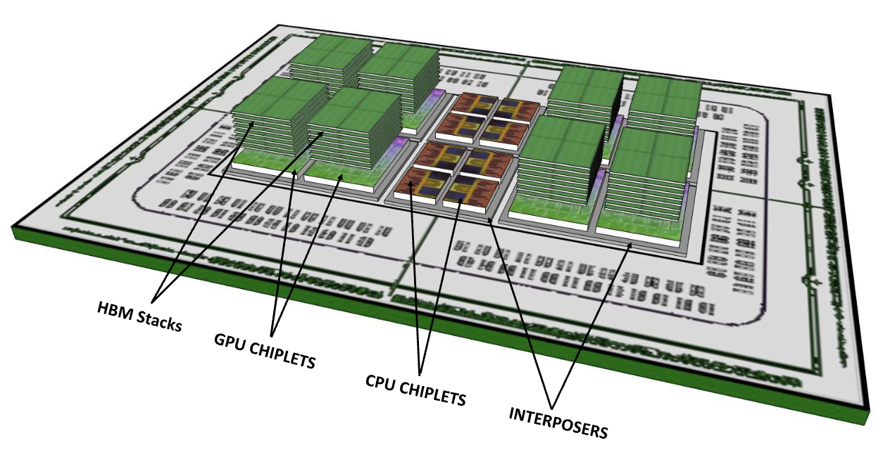
Modern AI accelerators, such as AMD’s Instinct MI300, take this approach by integrating multiple compute chiplets alongside memory chiplets, linked by high-speed die-to-die interconnects (Kannan, Dubey, and Horowitz 2023). This modular design allows manufacturers to bypass the manufacturing limits of monolithic chips while still achieving high-density compute.
Kannan, Harish, Pradeep Dubey, and Mark Horowitz. 2023. “Chiplet-Based Architectures: The Future of AI Accelerators.” IEEE Micro 43 (1): 46–55. https://doi.org/10.1109/MM.2022.1234567.
32 Memory Coherence: Ensuring all processors in a system see the same consistent view of shared memory when multiple cores/chips access the same data. Traditional cache coherence protocols like MESI add 10-50 ns latency for multi-core CPUs. For AI accelerators with thousands of cores, coherence becomes prohibitively expensive—most ML hardware instead uses explicit memory management where programmers control data placement and synchronization manually.
However, even within a single package, scaling is not without challenges. Inter-chiplet communication latency, memory coherence32, and thermal management become critical factors as more chiplets are integrated. Unlike traditional multi-chip systems, chiplet-based designs must carefully balance latency-sensitive workloads across multiple dies without introducing excessive bottlenecks.
Multi-GPU Systems
Beyond chiplet-based designs, AI workloads often require multiple discrete GPUs working together. In multi-GPU systems, each accelerator has its own dedicated memory and compute resources, but they must efficiently share data and synchronize execution.
A common example is NVIDIA DGX systems, which integrate multiple GPUs connected via NVLink or PCIe. This architecture enables workloads to be split across GPUs, typically using data parallelism (where each GPU processes a different batch of data) or model parallelism (where different GPUs handle different parts of a neural network) (Ben-Nun and Hoefler 2019). These parallelization strategies are explored in depth in Chapter 8: AI Training.
Ben-Nun, Tal, and Torsten Hoefler. 2019. “Demystifying Parallel and Distributed Deep Learning: An in-Depth Concurrency Analysis.” ACM Computing Surveys 52 (4): 1–43. https://doi.org/10.1145/3320060.
As illustrated in Figure 10, NVSwitch interconnects enable high-speed communication between GPUs, reducing bottlenecks in distributed training. However, scaling up the number of GPUs introduces fundamental distributed coordination challenges that become the dominant performance constraint. The arithmetic intensity of transformer training (0.5-2 FLOPS/byte) forces frequent gradient synchronization across GPUs, where AllReduce operations must aggregate 175 billion parameters in GPT-3 scale models. NVSwitch provides 600 GB/s bidirectional bandwidth, but even this substantial interconnect becomes bandwidth-bound when 8 H100 GPUs simultaneously exchange gradients, creating a 4.8 TB/s aggregate demand that exceeds available capacity. The coordination complexity compounds exponentially—while two GPUs require a single communication channel, eight GPUs need 28 interconnect paths, and fault tolerance requirements mandate redundant communication patterns. Memory consistency protocols further complicate coordination as different GPUs may observe weight updates at different times, requiring sophisticated synchronization primitives that can add 10-50μs latency per training step—seemingly small delays that aggregate to hours of training time across million-iteration runs.

Communication Overhead and Amdahl’s Law Analysis
The fundamental limitation of distributed AI training stems from Amdahl’s Law, which quantifies how communication overhead constrains parallel speedup regardless of available compute power. For distributed neural network training, communication overhead during gradient synchronization creates a sequential bottleneck that limits scalability even with infinite parallelism.
The maximum speedup achievable with distributed training is bound by Amdahl’s Law: \[ \text{Speedup} = \frac{1}{(1-P) + \frac{P}{N}} \] where \(P\) is the fraction of work that can be parallelized and \(N\) is the number of processors. However, for AI training, communication overhead introduces additional sequential time: \[ \text{Speedup}_{\text{AI}} = \frac{1}{(1-P) + \frac{P}{N} + \frac{C}{N}} \] where \(C\) represents the communication overhead fraction.
Consider training a 175 B parameter model with 1000 H100 GPUs as a concrete example:
- Computation time per iteration: 100 ms of forward/backward passes
- Communication time: AllReduce of 175 B parameters (700 GB in FP32) across 1000 GPUs
- Available bandwidth: 600 GB/s per NVSwitch link
- Communication overhead: \(\frac{700\text{GB}}{600\text{GB/s}} \times \log_2(1000) \approx 11.6\text{ms}\)
Even if only 5% of training requires communication (P = 0.95), the maximum speedup is: \[ \text{Speedup} = \frac{1}{0.05 + \frac{0.95}{1000} + \frac{0.116}{100}} \approx 8.3\text{x} \]
This demonstrates why adding more GPUs beyond ~100 provides diminishing returns for large model training.
Communication requirements scale superlinearly with model size and linearly with the number of parameters. Modern transformer models require gradient synchronization across all parameters during each training step:
- GPT-3 (175 B parameters): 700 GB gradient exchange per step
- GPT-4 (estimated 1.8 T parameters): ~7 TB gradient exchange per step
- Future 10 T parameter models: ~40 TB gradient exchange per step
Even with advanced interconnects like NVLink 4.0 (1.8 TB/s), gradient synchronization for 10 T parameter models would require 22+ seconds per training step, making distributed training impractical without algorithmic innovations like gradient compression or asynchronous updates.
Multi-GPU systems face additional bottlenecks from memory bandwidth competition. When 8 H100 GPUs simultaneously access HBM during gradient computation, the effective memory bandwidth per GPU drops from 3.35 TB/s to approximately 2.1 TB/s due to memory controller contention and NUMA effects. This 37% reduction in memory performance compounds communication overhead, further limiting scalability.
Understanding Amdahl’s Law guides optimization strategies:
- Gradient Compression: Reduce communication volume by 10-100\(\times\) through sparsification and quantization
- Pipeline Parallelism: Overlap communication with computation to hide gradient synchronization latency
- Model Parallelism: Partition models across devices to reduce gradient synchronization requirements
- Asynchronous Updates: Relax consistency requirements to eliminate synchronization barriers
These techniques modify the effective value of \(P\) and \(C\) in Amdahl’s equation, enabling better scaling behavior at the cost of algorithmic complexity.
TPU Pods
As models and datasets continue to expand, training and inference workloads must extend beyond single-server configurations. This scaling requirement has led to the development of sophisticated distributed systems where multiple accelerators communicate across networks. Google’s TPU Pods represent a pioneering approach to this challenge, interconnecting hundreds of TPUs to function as a unified system (Norman P. Jouppi et al. 2020).
Jouppi, Norman P., Doe Hyun Yoon, George Kurian, Sheng Li, Nishant Patil, James Laudon, Cliff Young, and David Patterson. 2020. “A Domain-Specific Supercomputer for Training Deep Neural Networks.” Communications of the ACM 63 (7): 67–78. https://doi.org/10.1145/3360307.
The architectural design of TPU Pods differs fundamentally from traditional multi-GPU systems. While multi-GPU configurations typically rely on NVLink or PCIe connections within a single machine, TPU Pods employ high-bandwidth optical links to interconnect accelerators at data center scale. This design implements a 2D torus interconnect topology, enabling efficient data exchange between accelerators while minimizing communication bottlenecks as workloads scale across nodes.
The effectiveness of this architecture is demonstrated in its performance scaling capabilities. As illustrated in Figure 11, TPU Pod performance exhibits near-linear scaling when running ResNet-50, from quarter-pod to full-pod configurations. The system achieves a remarkable 33.0\(\times\) speedup when scaled to 1024 chips compared to a 16-TPU baseline. This scaling efficiency is particularly noteworthy in larger configurations, where performance continues to scale strongly even as the system expands from 128 to 1024 chips.
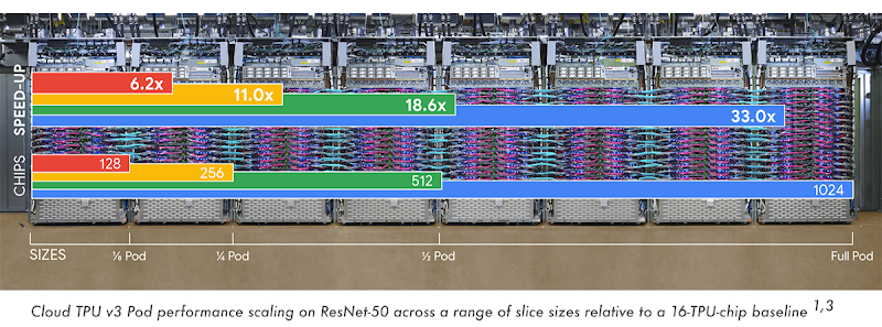
However, distributing AI workloads across an entire data center introduces distributed coordination challenges that fundamentally differ from single-node systems. The 2D torus interconnect, while providing high bisection bandwidth, creates communication bottlenecks when training large transformer models that require AllReduce operations across all 1,024 TPUs. Each parameter gradient must traverse multiple hops through the torus network, with worst-case communication requiring 32 hops between distant TPUs, creating latency penalties that compound with model size.
The distributed memory architecture exacerbates coordination complexity—unlike multi-GPU systems with shared host memory, each TPU node maintains independent memory spaces, forcing explicit data marshaling and synchronization protocols. Network partition tolerance becomes critical as optical link failures can split the pod into disconnected islands, requiring sophisticated consensus algorithms to maintain training consistency.
The energy cost of coordination also scales dramatically: moving data across the pod’s optical interconnect consumes 1000\(\times\) more energy than on-chip communication within individual TPUs, transforming distributed training into a careful balance between computation parallelism and communication efficiency where AllReduce bandwidth, not compute capacity, determines overall training throughput.
Wafer-Scale AI
At the frontier of AI scaling, wafer-scale33 integration represents a paradigm shift—abandoning traditional multi-chip architectures in favor of a single, massive AI processor. Rather than partitioning computation across discrete chips, this approach treats an entire silicon wafer as a unified compute fabric, eliminating the inefficiencies of inter-chip communication.
33 Wafer-Scale Integration: Using an entire 300 mm silicon wafer as a single processor instead of cutting it into individual chips. Cerebras WSE-3 contains 4 trillion transistors across 850,000 cores—125\(\times\) more than the largest GPUs. Manufacturing challenges include 100% yield requirements (solved with redundant cores) and cooling 23 kW of power. This approach eliminates inter-chip communication delays but costs $2-3 million per wafer versus $40,000 for equivalent GPU clusters.
Systems, Cerebras. 2021a. “The Wafer-Scale Engine 2: Scaling AI Compute Beyond GPUs.” Cerebras White Paper. https://cerebras.ai/product-chip/.
As shown in Figure 12, Cerebras’ Wafer-Scale Engine (WSE) processors break away from the historical transistor scaling trends of CPUs, GPUs, and TPUs. While these architectures have steadily increased transistor counts along an exponential trajectory, WSE introduces an entirely new scaling paradigm, integrating trillions of transistors onto a single wafer—far surpassing even the most advanced GPUs and TPUs. With WSE-3, this trajectory continues, pushing wafer-scale AI to unprecedented levels (Systems 2021a).
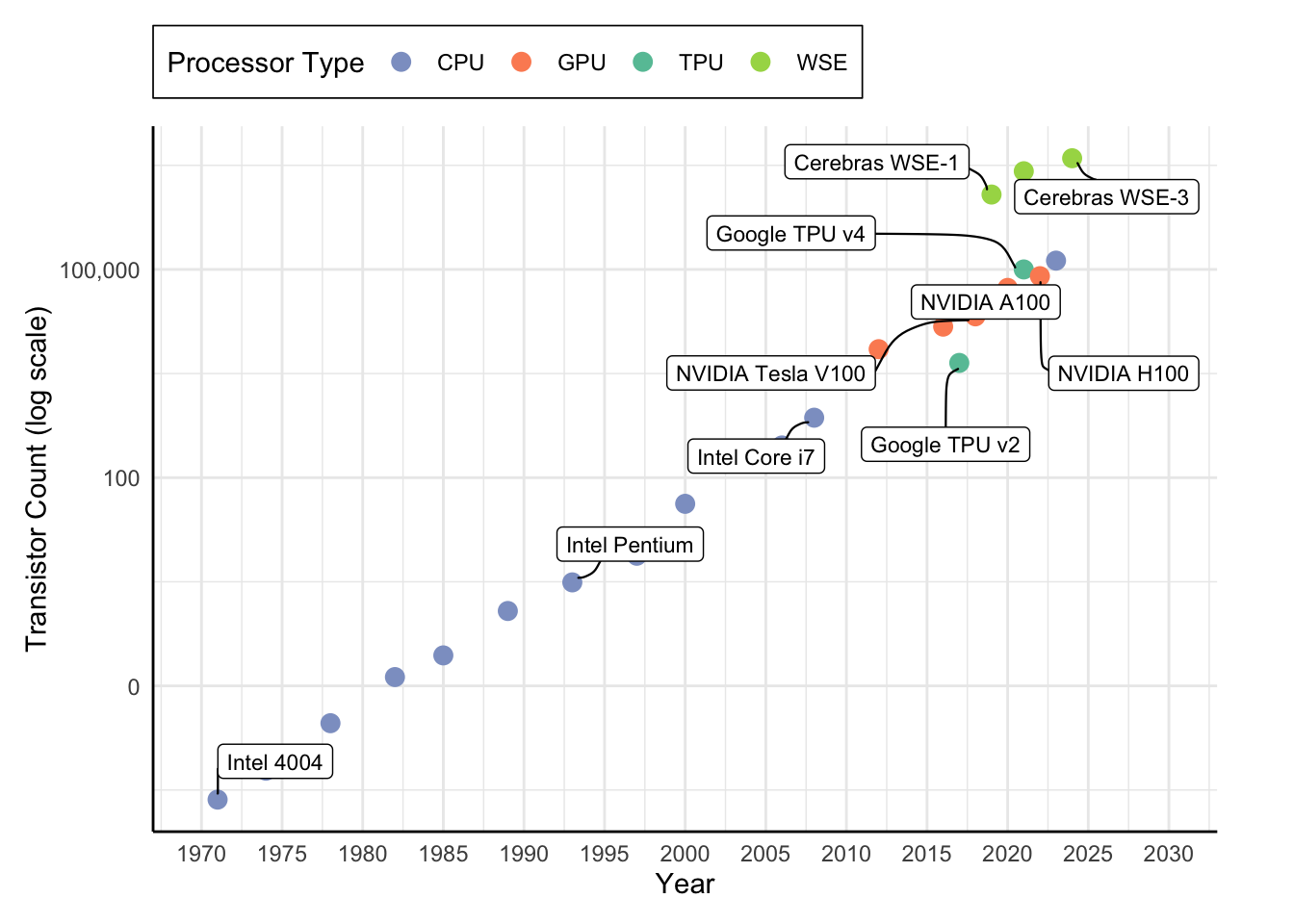
The fundamental advantage of wafer-scale AI is its ultra-fast, on-die communication. Unlike chiplets, GPUs, or TPU Pods, where data must traverse physical boundaries between separate devices, wafer-scale AI enables near-instantaneous data transfer across its vast compute array. This architecture drastically reduces communication latency, unlocking performance levels that are unachievable with conventional multi-chip systems.
However, achieving this level of integration introduces formidable engineering challenges. Thermal dissipation, fault tolerance, and manufacturing yield become major constraints when fabricating a processor of this scale. These sustainability challenges, including energy consumption and resource utilization, are examined in Chapter 18: Sustainable AI. Unlike distributed TPU systems, which mitigate failures by dynamically re-routing workloads, wafer-scale AI must incorporate built-in redundancy mechanisms to tolerate localized defects in the silicon. Successfully addressing these challenges is essential to realizing the full potential of wafer-scale computing as the next frontier in AI acceleration.
AI Systems Scaling Trajectory
Table 20 illustrates the progressive scaling of AI acceleration, from single-chip processors to increasingly complex architectures such as chiplet-based designs, multi-GPU systems, TPU Pods, and wafer-scale AI. Each step in this evolution introduces new challenges related to data movement, memory access, interconnect efficiency, and workload distribution. While chiplets enable modular scaling within a package, they introduce latency and memory coherence issues. Multi-GPU systems rely on high-speed interconnects like NVLink but face synchronization and communication bottlenecks. TPU Pods push scalability further by distributing workloads across clusters, yet they must contend with interconnect congestion and workload partitioning. At the extreme end, wafer-scale AI integrates an entire wafer into a single computational unit, presenting unique challenges in thermal management and fault tolerance.
| Scaling Approach | Key Feature | Challenges |
|---|---|---|
| Chiplets | Modular scaling within a package | Inter-chiplet latency, memory coherence |
| Multi-GPU | External GPU interconnects (NVLink) | Synchronization overhead, communication bottlenecks |
| TPU Pods | Distributed accelerator clusters | Interconnect congestion, workload partitioning |
| Wafer-Scale AI | Entire wafer as a single processor | Thermal dissipation, fault tolerance |
Computation and Memory Scaling Changes
As AI systems scale from single-chip accelerators to multi-chip architectures, the fundamental challenges in computation and memory evolve. In a single accelerator, execution is primarily optimized for locality—ensuring that computations are mapped efficiently to available processing elements while minimizing memory access latency. However, as AI systems extend beyond a single chip, the scope of these optimizations expands significantly. Computation must now be distributed across multiple accelerators, and memory access patterns become constrained by interconnect bandwidth and communication overhead.
Multi-chip Execution Mapping
In single-chip AI accelerators, computation placement is concerned with mapping workloads to PEs, vector units, and tensor cores. Mapping strategies aim to maximize data locality, ensuring that computations access nearby memory to reduce costly data movement.
As AI systems scale to multi-chip execution, computation placement must consider several critical factors. Workloads need to be partitioned across multiple accelerators, which requires explicit coordination of execution order and dependencies. This division is essential due to the inherent latency associated with cross-chip communication, which contrasts sharply with single-chip systems that benefit from shared on-chip memory. Accordingly, computation scheduling must be interconnect-aware to manage these delays effectively. Additionally, achieving load balancing across accelerators is vital; an uneven distribution of tasks can result in some accelerators remaining underutilized while others operate at full capacity, ultimately hindering overall system performance.
For example, in multi-GPU training, computation mapping must ensure that each GPU has a balanced portion of the workload while minimizing expensive cross-GPU communication. Similarly, in TPU Pods, mapping strategies must align with the torus interconnect topology, ensuring that computation is placed to minimize long-distance data transfers.
Thus, while computation placement in single-chip systems is a local optimization problem, in multi-chip architectures, it becomes a global optimization challenge where execution efficiency depends on minimizing inter-chip communication and balancing workload distribution.
Distributed Access Memory Allocation
Memory allocation strategies in single-chip AI accelerators are designed to minimize off-chip memory accesses by using on-chip caches, SRAM, and HBM. Techniques such as tiling, data reuse, and kernel fusion ensure that computations make efficient use of fast local memory.
In multi-chip AI systems, each accelerator manages its own local memory, which necessitates the explicit allocation of model parameters, activations, and intermediate data across the devices. Unlike single-chip execution where data is fetched once and reused, multi-chip setups require deliberate strategies to minimize redundant data transfers, as data must be communicated between accelerators. Additionally, when overlapping data is processed by multiple accelerators, the synchronization of shared data can introduce significant overhead that must be carefully managed to ensure efficient execution.
For instance, in multi-GPU deep learning, gradient synchronization across GPUs is a memory-intensive operation that must be optimized to avoid network congestion (Shallue et al. 2019). In wafer-scale AI, memory allocation must account for fault tolerance and redundancy mechanisms, ensuring that defective regions of the wafer do not disrupt execution.
Shallue, Christopher J, Jaehoon Lee, Joseph Antognini, Jascha Sohl-Dickstein, Roy Frostig, and George E Dahl. 2019. “Measuring the Effects of Data Parallelism on Neural Network Training.” Journal of Machine Learning Research 20: 1–49. http://jmlr.org/papers/v20/18-789.html.
Thus, while memory allocation in single-chip accelerators focuses on local cache efficiency, in multi-chip architectures, it must be explicitly coordinated across accelerators to balance memory bandwidth, minimize redundant transfers, and reduce synchronization overhead.
Data Movement Constraints
In single-chip AI accelerators, data movement optimization is largely focused on minimizing on-chip memory access latency. Techniques such as weight stationarity, input stationarity, and tiling ensure that frequently used data remains close to the execution units, reducing off-chip memory traffic.
In multi-chip architectures, data movement transcends being merely an intra-chip issue and becomes a significant system-wide bottleneck. Scaling introduces several critical challenges, foremost among them being inter-chip bandwidth constraints; communication links such as PCIe, NVLink, and TPU interconnects operate at speeds that are considerably slower than those of on-chip memory accesses. Additionally, when accelerators share model parameters or intermediate computations, the resulting data synchronization overhead, which encompass latency and contention, can markedly impede execution. Finally, optimizing collective communication is essential for workloads that require frequent data exchanges, such as gradient updates in deep learning training, where minimizing synchronization penalties is imperative for achieving efficient system performance.
For example, in TPU Pods, systolic execution models ensure that data moves in structured patterns, reducing unnecessary off-chip transfers. In multi-GPU inference, techniques like asynchronous data fetching and overlapping computation with communication help mitigate inter-chip latency.
Thus, while data movement optimization in single-chip systems focuses on cache locality and tiling, in multi-chip architectures, the primary challenge is reducing inter-chip communication overhead to maximize efficiency.
Compilers and Runtimes Adaptation
As AI acceleration extends beyond a single chip, compilers and runtimes must adapt to manage computation placement, memory organization, and execution scheduling across multiple accelerators. The fundamental principles of locality, parallelism, and efficient scheduling remain essential, but their implementation requires new strategies for distributed execution.
One of the primary challenges in scaling AI execution is computation placement. In a single-chip accelerator, workloads are mapped to processing elements, vector units, and tensor cores with an emphasis on minimizing on-chip data movement and maximizing parallel execution. However, in a multi-chip system, computation must be partitioned hierarchically, where workloads are distributed not just across cores within a chip, but also across multiple accelerators. Compilers handle this by implementing interconnect-aware scheduling, optimizing workload placement to minimize costly inter-chip communication.
Similarly, memory management evolves as scaling extends beyond a single accelerator. In a single-chip system, local caching, HBM reuse, and efficient tiling strategies ensure that frequently accessed data remains close to computation units. However, in a multi-chip system, each accelerator has its own independent memory, requiring explicit memory partitioning and coordination. Compilers optimize memory layouts for distributed execution, while runtimes introduce data prefetching and caching mechanisms to reduce inter-chip memory access overhead.
Beyond computation and memory, data movement becomes a major bottleneck at scale. In a single-chip accelerator, efficient on-chip caching and minimized DRAM accesses ensure that data is reused efficiently. However, in a multi-chip system, communication-aware execution becomes critical, requiring compilers to generate execution plans that overlap computation with data transfers. Runtimes handle inter-chip synchronization, ensuring that workloads are not stalled by waiting for data to arrive from remote accelerators.
Finally, execution scheduling must be extended for global coordination. In single-chip AI execution, scheduling is primarily concerned with parallelism and maximizing compute occupancy within the accelerator. However, in a multi-chip system, scheduling must balance workload distribution across accelerators while taking interconnect bandwidth and synchronization latency into account. Runtimes manage this complexity by implementing adaptive scheduling strategies that dynamically adjust execution plans based on system state and network congestion.
Table 21 summarizes these key adaptations, highlighting how compilers and runtimes extend their capabilities to efficiently support multi-chip AI execution.
Thus, while the fundamentals of AI acceleration remain intact, compilers and runtimes must extend their functionality to operate efficiently across distributed systems. The next section will explore how mapping strategies evolve to further optimize multi-chip AI execution.
| Aspect | Single-Chip AI Accelerator | Multi-Chip AI System & How Compilers/Runtimes Adapt |
|---|---|---|
| Computation Placement | Local PEs, tensor cores, vector units | Hierarchical mapping, interconnect-aware scheduling |
| Memory Management | Caching, HBM reuse, local tiling | Distributed allocation, prefetching, caching |
| Data Movement | On-chip reuse, minimal DRAM access | Communication-aware execution, overlap transfers |
| Execution Scheduling | Parallelism, compute occupancy | Global scheduling, interconnect-aware balancing |
Execution Models Adaptation
As AI accelerators scale beyond a single chip, execution models must evolve to account for the complexities introduced by distributed computation, memory partitioning, and inter-chip communication. In single-chip accelerators, execution is optimized for local processing elements, with scheduling strategies that balance parallelism, locality, and data reuse. However, in multi-chip AI systems, execution must now be coordinated across multiple accelerators, introducing new challenges in workload scheduling, memory coherence, and interconnect-aware execution.
This section explores how execution models change as AI acceleration scales, focusing on scheduling, memory coordination, and runtime management in multi-chip systems.
Cross-Accelerator Scheduling
In single-chip AI accelerators, execution scheduling is primarily aimed at optimizing parallelism within the processor. This involves ensuring that workloads are effectively mapped to tensor cores, vector units, and special function units by employing techniques designed to enhance data locality and resource utilization. For instance, static scheduling uses a predetermined execution order that is carefully optimized for locality and reuse, while dynamic scheduling adapts in real time to variations in workload demands. Additionally, pipeline execution divides computations into stages, thereby maximizing hardware utilization by maintaining a continuous flow of operations.
In contrast, scheduling in multi-chip architectures must address the additional challenges posed by inter-chip dependencies. Workload partitioning in such systems involves distributing tasks across various accelerators such that each receives an optimal share of the workload, all while minimizing the overhead caused by excessive communication. Interconnect-aware scheduling is essential to align execution timing with the constraints of inter-chip bandwidth, thus preventing performance stalls. Latency hiding techniques also play a critical role, as they enable the overlapping of computation with communication, effectively reducing waiting times.
For example, in multi-GPU inference scenarios, execution scheduling is implemented in a way that allows data to be prefetched concurrently with computation, thereby mitigating memory stalls. Similarly, TPU Pods leverage the systolic array model to tightly couple execution scheduling with data flow, ensuring that each TPU core receives its required data precisely when needed. Therefore, while single-chip execution scheduling is focused largely on maximizing internal parallelism, multi-chip systems require a more holistic approach that explicitly manages communication overhead and synchronizes workload distribution across accelerators.
Cross-Accelerator Coordination
In single-chip AI accelerators, memory coordination is managed through sophisticated local caching strategies that keep frequently used data in close proximity to the execution units. Techniques such as tiling, kernel fusion, and data reuse are employed to reduce the dependency on slower memory hierarchies, thereby enhancing performance and reducing latency.
In contrast, multi-chip architectures present a distributed memory coordination challenge that necessitates more deliberate management. Each accelerator in such a system possesses its own independent memory, which must be organized through explicit memory partitioning to minimize cross-chip data accesses. Additionally, ensuring consistency and synchronization of shared data across accelerators is essential to maintain computational correctness. Efficient communication mechanisms must also be implemented to schedule data transfers in a way that limits overhead associated with synchronization delays.
For instance, in distributed deep learning training, model parameters must be synchronized across multiple GPUs using methods such as all-reduce, where gradients are aggregated across accelerators while reducing communication latency. In wafer-scale AI, memory coordination must further address fault-tolerant execution, ensuring that defective areas do not compromise overall system performance. Consequently, while memory coordination in single-chip systems is primarily concerned with cache optimization, multi-chip architectures require management of distributed memory access, synchronization, and communication to achieve efficient execution.
Cross-Accelerator Execution Management
Execution in single-chip AI accelerators is managed by AI runtimes that handle workload scheduling, memory allocation, and hardware execution. These runtimes optimize execution at the kernel level, ensuring that computations are executed efficiently within the available resources.
In multi-chip AI systems, runtimes must incorporate a strategy for distributed execution orchestration. This approach ensures that both computation and memory access are seamlessly coordinated across multiple accelerators, enabling efficient utilization of hardware resources and minimizing bottlenecks associated with data transfers.
These systems require robust mechanisms for cross-chip workload synchronization. Careful management of dependencies and timely coordination between accelerators are essential to prevent stalls in execution that may arise from delays in inter-chip communication. Such synchronization is critical for maintaining the flow of computation, particularly in environments where latency can significantly impact overall performance.
Finally, adaptive execution models play a pivotal role in contemporary multi-chip architectures. These models dynamically adjust execution plans based on current hardware availability and communication constraints, ensuring that the system can respond to changing conditions and optimize performance in real time. Together, these strategies provide a resilient framework for managing the complexities of distributed AI execution.
For example, in Google’s TPU Pods, the TPU runtime is responsible for scheduling computations across multiple TPU cores, ensuring that workloads are executed in a way that minimizes communication bottlenecks. In multi-GPU frameworks like PyTorch and TensorFlow, runtime execution must synchronize operations across GPUs, ensuring that data is transferred efficiently while maintaining execution order.
Thus, while single-chip runtimes focus on optimizing execution within a single processor, multi-chip runtimes must handle system-wide execution, balancing computation, memory, and interconnect performance.
Computation Placement Adaptation
As AI systems expand beyond single-chip execution, computation placement must adapt to account for inter-chip workload distribution and interconnect efficiency. In single-chip accelerators, compilers optimize placement by mapping workloads to tensor cores, vector units, and PEs, ensuring maximum parallelism while minimizing on-chip data movement. However, in multi-chip systems, placement strategies must address interconnect bandwidth constraints, synchronization latency, and hierarchical workload partitioning across multiple accelerators.
Table 22 highlights these adaptations. To reduce expensive cross-chip communication, compilers now implement interconnect-aware workload partitioning, strategically assigning computations to accelerators based on communication cost. For instance, in multi-GPU training, compilers optimize placement to minimize NVLink or PCIe traffic, whereas TPU Pods leverage the torus interconnect topology to enhance data exchanges.
| Aspect | Single-Chip AI Accelerator | Multi-Chip AI System & How Compilers/Runtimes Adapt |
|---|---|---|
| Computation Placement | Local PEs, tensor cores, vector units | Hierarchical mapping, interconnect-aware scheduling |
| Workload Distribution | Optimized within a single chip | Partitioning across accelerators, minimizing inter-chip communication |
| Synchronization | Managed within local execution units | Runtimes dynamically balance workloads, adjust execution plans |
Runtimes complement this by dynamically managing execution workloads, adjusting placement in real-time to balance loads across accelerators. Unlike static compilation, which assumes a fixed hardware topology, AI runtimes continuously monitor system conditions and migrate tasks as needed to prevent bottlenecks. This ensures efficient execution even in environments with fluctuating workload demands or varying hardware availability.
Thus, computation placement at scale builds upon local execution optimizations while introducing new challenges in inter-chip coordination, communication-aware execution, and dynamic load balancing—challenges that extend to how memory hierarchies must adapt to support efficient execution across multi-chip architectures.
Heterogeneous SoC AI Acceleration
The multi-chip architectures examined in previous sections focused primarily on maximizing computational throughput for data center workloads, where power budgets extend to kilowatts and cooling infrastructure supports rack-scale deployments. However, the hardware acceleration principles established—specialized compute units, memory hierarchy optimization, and workload mapping strategies—must adapt dramatically when deploying AI systems in mobile and edge environments. A smartphone operates within a 2 to 5 watt power budget, autonomous vehicles require deterministic real-time guarantees, and IoT sensors must function for years on battery power. These constraints necessitate heterogeneous System-on-Chip (SoC) architectures that coordinate multiple specialized processors within a single chip while meeting stringent power, thermal, and latency requirements fundamentally different from data center deployments.
The mobile AI revolution has fundamentally transformed how we think about AI acceleration, moving beyond homogeneous data center architectures to heterogeneous System-on-Chip (SoC) designs that coordinate multiple specialized processors. Modern smartphones, automotive systems, and IoT devices integrate CPU cores, GPU shaders, digital signal processors (DSPs), and dedicated neural processing units (NPUs) within a single chip, requiring sophisticated orchestration to achieve optimal performance under strict power and thermal constraints.
Mobile SoC Architecture Evolution
Qualcomm’s Snapdragon AI Engine exemplifies heterogeneous computing for mobile AI, coordinating Kryo CPU cores, Adreno GPU, Hexagon DSP, and dedicated NPU34 across a shared memory hierarchy. The Snapdragon 8 Gen 3 achieves 73 TOPS through intelligent workload distribution—computer vision kernels execute on the GPU’s parallel shaders, audio processing leverages the DSP’s specialized arithmetic units, while transformer attention mechanisms utilize the NPU’s optimized matrix engines. This coordination requires millisecond-precision scheduling to meet real-time constraints while managing thermal throttling and battery life optimization.
34 Neural Processing Unit (NPU): Specialized processors designed specifically for neural network inference, distinct from general-purpose GPUs. Apple introduced the first consumer NPU in the A11 chip (2017), achieving 600 billion operations per second while consuming less than 1 watt. Modern NPUs like Apple’s M3 Neural Engine deliver 18 TOPS for on-device AI tasks like real-time image processing, voice recognition, and computational photography. NPUs excel at low-power, fixed-function AI workloads but lack the programmability of GPUs for diverse ML research.
While Qualcomm’s approach emphasizes diverse processor specialization, Apple’s vertically integrated strategy demonstrates how tight hardware-software co-design enables even more sophisticated heterogeneous execution. The M2 chip’s 16-core Neural Engine (15.8 TOPS) coordinates with the 10-core GPU and 8-core CPU through a unified memory architecture that eliminates data copying overhead. The Neural Engine’s specialized matrix multiplication units handle transformer layers, while the GPU’s Metal Performance Shaders accelerate convolutional operations, and the CPU manages control flow and dynamic layer selection. This fine-grained coordination enables real-time language translation and on-device image generation while maintaining millisecond response times.
Beyond these vertically integrated solutions from Qualcomm and Apple, ARM’s IP licensing model offers a fundamentally different approach that enables SoC designers to customize processor combinations based on target applications. The Mali-G78 GPU’s 24 cores can be paired with Ethos-N78 NPU for balanced general-purpose and AI acceleration, while the Cortex-M55 microcontroller integrates Ethos-U55 microNPU for ultra-low-power edge applications. This modular flexibility allows automotive SoCs to emphasize deterministic real-time processing while smartphone SoCs optimize for interactive performance and battery efficiency.
Strategies for Dynamic Workload Distribution
With multiple specialized processors available on heterogeneous SoCs, the critical challenge becomes intelligently distributing neural network operations across these resources to maximize performance while respecting power and latency constraints.
Modern neural networks require intelligent partitioning across heterogeneous processors based on operation characteristics and current system state. Convolutional layers with regular data access patterns typically execute efficiently on GPU shader cores, while fully connected layers with irregular sparsity patterns may perform better on general-purpose CPU cores with large caches. Attention mechanisms in transformers benefit from NPU matrix engines when sequences are long, but may execute more efficiently on CPU when sequence lengths are small due to the NPU setup overhead.
Beyond static operation-to-processor mapping, heterogeneous SoCs implement dynamic processor selection based on multiple constraints:
- Power Budget: During battery operation, the system may route computations to lower-power DSP cores rather than high-performance GPU cores
- Thermal State: When approaching thermal limits, workloads shift from power-hungry NPU to more efficient CPU execution
- Latency Requirements: Safety-critical automotive applications prioritize deterministic CPU execution over potentially faster but variable NPU processing
- Concurrent Workload Interference: Multiple AI applications may require load balancing across available processors to maintain Quality of Service
Compounding the processor selection challenge, shared memory architectures require sophisticated arbitration when multiple processors access LPDDR simultaneously. The Snapdragon 8 Gen 3’s memory controller implements priority-based scheduling where camera processing receives higher priority than background AI tasks, ensuring real-time video processing while background neural networks adapt their execution patterns to available memory bandwidth. This arbitration becomes critical during memory-intensive operations like large language model inference, where parameter streaming from DRAM must be carefully coordinated across processors.
Power and Thermal Management
Mobile AI workloads must maintain high performance while operating within strict power budgets and thermal envelopes—constraints that require sophisticated coordination across heterogeneous processors.
Heterogeneous SoCs implement coordinated DVFS across multiple processors to optimize the power-performance envelope. When one processor increases frequency to meet latency demands, the system may reduce voltage on other processors to maintain total power budget. This coordination becomes complex in AI workloads where computational phases may shift rapidly between processors—the system must predict upcoming workload transitions to preemptively adjust operating points while avoiding voltage/frequency oscillations that degrade efficiency.
When DVFS alone cannot maintain the power envelope, mobile SoCs implement thermal throttling through intelligent task migration rather than simple frequency reduction. When the NPU approaches thermal limits during intensive neural network processing, the runtime system can migrate layers to the GPU or CPU while maintaining computational throughput. This approach preserves performance during thermal events, though it requires sophisticated workload characterization to predict execution time and power consumption across different processors.
Beyond real-time power and thermal management, mobile AI systems must also adapt their computational strategies based on battery state and charging status. During low battery conditions, the system may switch from high-accuracy models to efficient approximations, migrate workloads from power-hungry NPU to energy-efficient DSP, or reduce inference frequency while maintaining application responsiveness. Conversely, during charging, the system can enable higher-performance models and increase processing frequency to deliver enhanced user experiences.
Automotive Heterogeneous AI Systems
Automotive applications introduce unique heterogeneous computing challenges that combine mobile-style power efficiency with hard real-time guarantees and functional safety requirements—a combination that demands fundamentally different architectural approaches.
Automotive SoCs must guarantee deterministic inference latency for safety-critical functions while supporting advanced driver assistance systems (ADAS). The Snapdragon Ride platform coordinates multiple AI accelerators across safety domains—redundant processing elements ensure functional safety compliance while high-performance accelerators handle perception, planning, and control algorithms. This architecture requires temporal isolation between safety-critical and convenience functions, implemented through hardware partitioning and time-triggered scheduling.
These safety requirements become even more complex when considering that modern vehicles integrate multiple AI-enabled SoCs for different domains—vision processing SoCs handle camera-based perception, radar processing SoCs manage RF sensor data, while central compute platforms coordinate high-level decision making. These distributed systems must maintain temporal coherence across sensor modalities with microsecond-precision timing, requiring specialized inter-SoC communication protocols and distributed synchronization mechanisms.
Extending beyond the vehicle’s internal sensors, vehicle-to-everything (V2X) communication adds another layer of heterogeneous processing where AI algorithms must coordinate local sensor processing with information received from other vehicles and infrastructure. This requires ultra-low latency processing chains where 5G modems, AI accelerators, and control systems operate within millisecond deadlines while maintaining functional safety requirements.
Software Stack Challenges
The architectural sophistication of heterogeneous SoCs creates substantial software development challenges that span programming models, memory management, and runtime optimization.
Programming heterogeneous SoCs requires frameworks that abstract processor differences while exposing performance-critical optimization opportunities. OpenCL and Vulkan provide cross-processor execution, but achieving optimal performance requires processor-specific optimizations that complicate portable development. Modern ML frameworks like TensorFlow Lite and PyTorch Mobile implement automatic processor selection, but developers still need to understand heterogeneous execution patterns to achieve optimal results.
Complicating the programming challenge further, heterogeneous SoCs with shared memory architectures require sophisticated memory management that considers processor-specific caching behaviors, memory access patterns, and coherency requirements. CPU caches may interfere with GPU memory access patterns, while NPU direct memory access (DMA) operations must be synchronized with CPU cache operations to maintain data consistency.
To address the complexity of manual optimization across these dimensions, advanced heterogeneous SoCs implement machine learning-based runtime optimization that learns from execution patterns to improve processor selection, thermal management, and power optimization. These systems collect telemetry on workload characteristics, processor utilization, and power consumption to build models that predict optimal execution strategies for new workloads.
This heterogeneous approach to AI acceleration represents the future of computing, where no single processor architecture can optimally handle the diverse computational patterns in modern AI applications. Understanding these coordination challenges is essential for developing efficient mobile AI systems that deliver high performance while meeting the strict power, thermal, and real-time constraints of edge deployment scenarios.
However, the complexity of these heterogeneous systems creates numerous opportunities for misconception and suboptimal design decisions. The following fallacies and pitfalls highlight common misunderstandings that can undermine acceleration strategies.
Fallacies and Pitfalls
Hardware acceleration involves complex interactions between specialized architectures, software stacks, and workload characteristics that create significant opportunities for misunderstanding optimal deployment strategies. The impressive performance numbers often associated with AI accelerators can mask important constraints and trade-offs that determine real-world effectiveness across different deployment scenarios.
Fallacy: More specialized hardware always provides better performance than general-purpose alternatives.
This belief assumes that specialized accelerators automatically outperform general-purpose processors for all AI workloads. Specialized hardware achieves peak performance only when workloads match the architectural assumptions and optimization targets. Models with irregular memory access patterns, small batch sizes, or dynamic computation graphs may perform better on flexible general-purpose processors than on specialized accelerators designed for dense, regular computations. The overhead of data movement, format conversion, and synchronization can eliminate the benefits of specialized computation. Effective hardware selection requires matching workload characteristics to architectural strengths rather than assuming specialization always wins.
Pitfall: Ignoring memory bandwidth limitations when selecting acceleration strategies.
Many practitioners focus on computational throughput metrics without considering memory bandwidth constraints that often limit real-world performance. AI accelerators with impressive computational capabilities can be severely bottlenecked by insufficient memory bandwidth, leading to poor hardware utilization. The ratio between computation intensity and memory access requirements determines whether an accelerator can achieve its theoretical performance. This oversight leads to expensive hardware deployments that fail to deliver expected performance improvements because the workload is memory-bound rather than compute-bound.
Fallacy: Hardware acceleration benefits scale linearly with additional accelerators.
This misconception drives teams to expect proportional performance gains when adding more accelerators to their systems. Multi-accelerator setups introduce communication overhead, synchronization costs, and load balancing challenges that can severely limit scaling efficiency. Small models may not provide enough parallel work to utilize multiple accelerators effectively, while large models may be limited by communication bandwidth between devices. Distributed training and inference face additional challenges from gradient aggregation, model partitioning, and coordination overhead that create non-linear scaling relationships.
Pitfall: Vendor-specific optimizations without considering long-term portability and flexibility.
Organizations often optimize exclusively for specific hardware vendors to achieve maximum performance without considering the implications for system flexibility and future migration. Deep integration with vendor-specific libraries, custom kernels, and proprietary optimization tools creates lock-in that complicates hardware upgrades, vendor changes, or multi-vendor deployments. While vendor-specific optimizations can provide significant performance benefits, they should be balanced against the need for system portability and the ability to adapt to evolving hardware landscapes. Maintaining some level of hardware abstraction preserves strategic flexibility while still capturing most performance benefits.
Summary
Hardware acceleration has emerged as the critical enabler that transforms machine learning from academic curiosity to practical reality, fundamentally reshaping how we design both computational systems and the algorithms that run on them. The evolution from general-purpose processors to specialized AI accelerators represents more than just incremental improvement—it reflects a paradigm shift toward domain-specific computing where hardware and software are co-designed to optimize specific computational patterns. The journey from CPUs through GPUs to specialized TPUs, NPUs, and wafer-scale systems demonstrates how understanding workload characteristics drives architectural innovation, creating opportunities for orders-of-magnitude performance improvements through targeted specialization.
The technical challenges of AI acceleration span multiple layers of the computing stack, from low-level memory hierarchy optimization to high-level compiler transformations and runtime orchestration. Memory bandwidth limitations create fundamental bottlenecks that require sophisticated techniques like data tiling, kernel fusion, and hierarchy-aware scheduling to overcome. Mapping neural network computations to hardware involves complex trade-offs between different dataflow patterns, memory allocation strategies, and execution scheduling approaches that must balance computational efficiency with resource utilization.
Building on these foundational concepts, the emergence of multi-chip and distributed acceleration systems introduces additional complexities around communication overhead, memory coherence, and workload partitioning that require careful system-level optimization.
Key Takeaways
- Specialized AI accelerators achieve performance gains through domain-specific architectures optimized for tensor operations and dataflow patterns
- Memory hierarchy management is often the primary bottleneck in AI acceleration, requiring sophisticated data movement optimization strategies
- Hardware-software co-design enables order-of-magnitude improvements by aligning algorithm characteristics with architectural capabilities
- Multi-chip scaling introduces distributed computing challenges that require new approaches to communication, synchronization, and resource management
The principles of hardware acceleration established here provide the foundation for understanding how benchmarking methodologies evaluate accelerator performance and how deployment strategies must account for hardware constraints and capabilities. As AI models continue growing in complexity and computational requirements, the ability to effectively leverage specialized hardware becomes increasingly critical for practical system deployment, influencing everything from energy efficiency and cost optimization to the feasibility of real-time inference and large-scale training across diverse application domains.