3 DL Primer
Resources: Slides, Videos, Exercises, Labs
This section briefly introduces deep learning, starting with an overview of its history, applications, and relevance to embedded AI systems. It examines the core concepts like neural networks, highlighting key components like perceptrons, multilayer perceptrons, activation functions, and computational graphs. The primer also briefly explores major deep learning architecture, contrasting their applications and uses. Additionally, it compares deep learning to traditional machine learning to equip readers with the general conceptual building blocks to make informed choices between deep learning and traditional ML techniques based on problem constraints, setting the stage for more advanced techniques and applications that will follow in subsequent chapters.
Understand the basic concepts and definitions of deep neural networks.
Recognize there are different deep learning model architectures.
Comparison between deep learning and traditional machine learning approaches across various dimensions.
Acquire the basic conceptual building blocks to dive deeper into advanced deep-learning techniques and applications.
3.1 Introduction
3.1.1 Definition and Importance
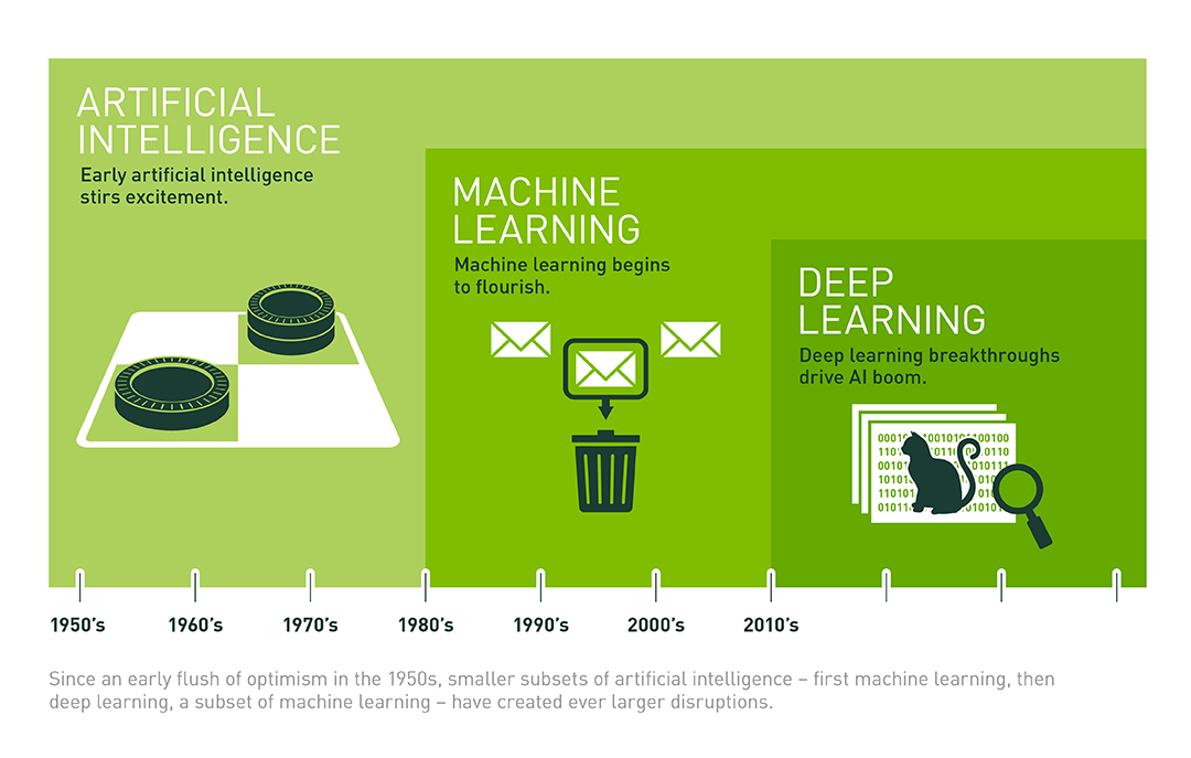
Deep learning, a specialized area within machine learning and artificial intelligence (AI), utilizes algorithms modeled after the structure and function of the human brain, known as artificial neural networks. This field is a foundational element in AI, driving progress in diverse sectors such as computer vision, natural language processing, and self-driving vehicles. Its significance in embedded AI systems is highlighted by its capability to handle intricate calculations and predictions, optimizing the limited resources in embedded settings. Figure 3.1 illustrates the chronological development and relative segmentation of the three fields.
3.1.2 Brief History of Deep Learning
The idea of deep learning has origins in early artificial neural networks. It has experienced several cycles of interest, starting with the introduction of the Perceptron in the 1950s (Rosenblatt 1957), followed by the invention of backpropagation algorithms in the 1980s (Rumelhart, Hinton, and Williams 1986).
The term “deep learning” became prominent in the 2000s, characterized by advances in computational power and data accessibility. Important milestones include the successful training of deep networks like AlexNet (Krizhevsky, Sutskever, and Hinton 2012) by Geoffrey Hinton, a leading figure in AI, and the renewed focus on neural networks as effective tools for data analysis and modeling.
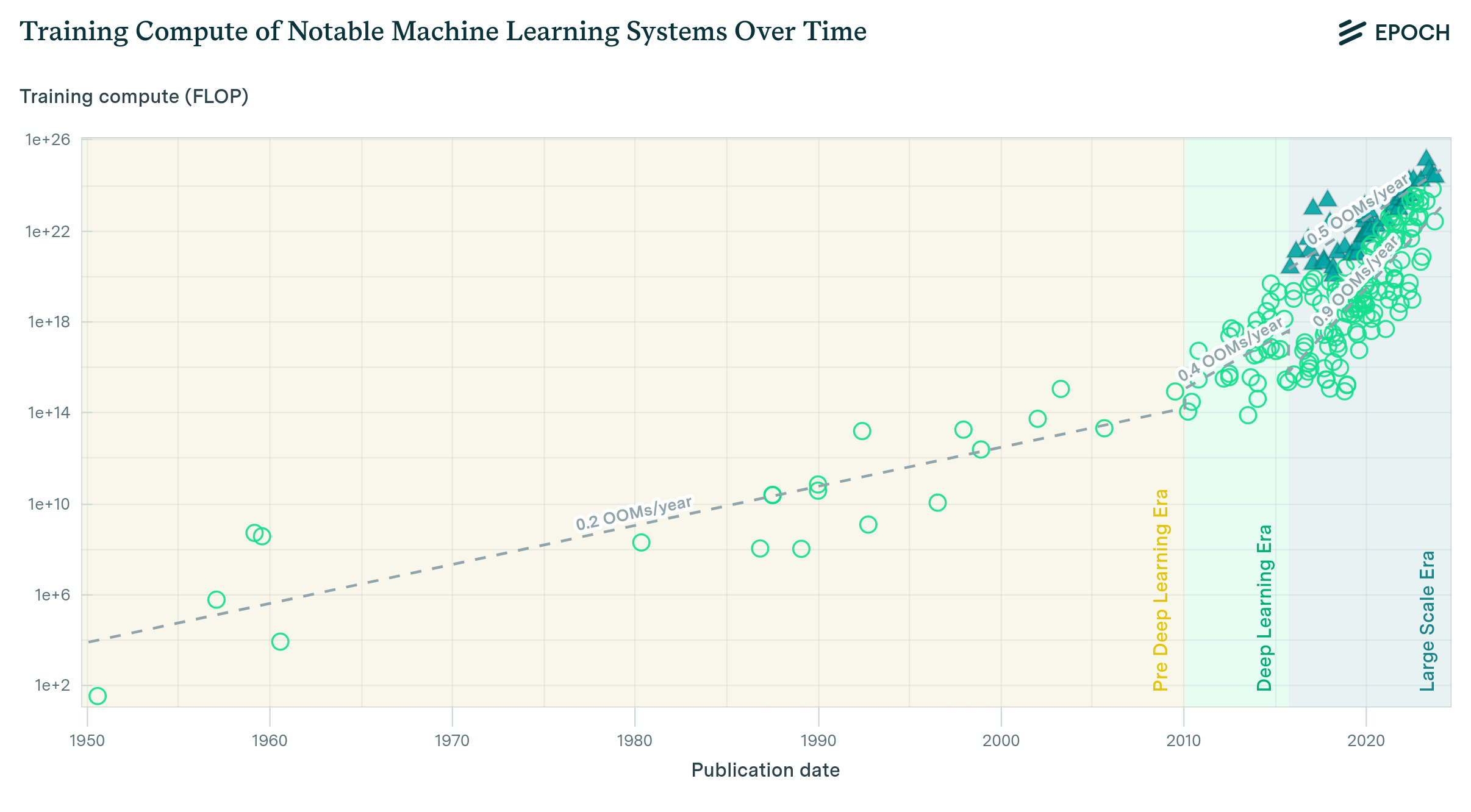
Deep learning has recently seen exponential growth, transforming various industries. Computational growth followed an 18-month doubling pattern from 1952 to 2010, which then accelerated to a 6-month cycle from 2010 to 2022, as shown in Figure 3.2. Concurrently, we saw the emergence of large-scale models between 2015 and 2022, appearing 2 to 3 orders of magnitude faster and following a 10-month doubling cycle.
Multiple factors have contributed to this surge, including advancements in computational power, the abundance of big data, and improvements in algorithmic designs. First, the growth of computational capabilities, especially the arrival of Graphics Processing Units (GPUs) and Tensor Processing Units (TPUs) (Jouppi et al. 2017), has significantly sped up the training and inference times of deep learning models. These hardware improvements have enabled the construction and training of more complex, deeper networks than what was possible in earlier years.
Second, the digital revolution has yielded a wealth of big data, offering rich material for deep learning models to learn from and excel in tasks such as image and speech recognition, language translation, and game playing. Large, labeled datasets have been key in refining and successfully deploying deep learning applications in real-world settings.
Additionally, collaborations and open-source efforts have nurtured a dynamic community of researchers and practitioners, accelerating advancements in deep learning techniques. Innovations like deep reinforcement learning, transfer learning, and generative artificial intelligence have broadened the scope of what is achievable with deep learning, opening new possibilities in various sectors, including healthcare, finance, transportation, and entertainment.
Organizations worldwide recognize deep learning’s transformative potential and invest heavily in research and development to leverage its capabilities in providing innovative solutions, optimizing operations, and creating new business opportunities. As deep learning continues its upward trajectory, it is set to redefine how we interact with technology, enhancing convenience, safety, and connectivity in our lives.
3.1.3 Applications of Deep Learning
Deep learning is extensively used across numerous industries today, and its transformative impact on society is evident. In finance, it powers stock market prediction, risk assessment, and fraud detection. For instance, deep learning algorithms can predict stock market trends, guide investment strategies, and improve financial decisions. In marketing, it drives customer segmentation, personalization, and content optimization. Deep learning analyzes consumer behavior and preferences to enable highly targeted advertising and personalized content delivery. In manufacturing, deep learning streamlines production processes and enhances quality control by continuously analyzing large volumes of data. This allows companies to boost productivity and minimize waste, leading to the production of higher quality goods at lower costs. In healthcare, machine learning aids in diagnosis, treatment planning, and patient monitoring. Similarly, deep learning can make medical predictions that improve patient diagnosis and save lives. The benefits are clear: machine learning predicts with greater accuracy than humans and does so much more quickly.
Deep learning enhances everyday products, such as strengthening Netflix’s recommender systems to provide users with more personalized recommendations. At Google, deep learning models have driven significant improvements in Google Translate, enabling it to handle over 100 languages. Autonomous vehicles from companies like Waymo, Cruise, and Motional have become a reality through the use of deep learning in their perception system. Additionally, Amazon employs deep learning at the edge in their Alexa devices to perform keyword spotting.
3.1.4 Relevance to Embedded AI
Embedded AI, the integration of AI algorithms directly into hardware devices, naturally gains from deep learning capabilities. Combining deep learning algorithms and embedded systems has laid the groundwork for intelligent, autonomous devices capable of advanced on-device data processing and analysis. Deep learning aids in extracting complex patterns and information from input data, which is essential in developing smart embedded systems, from household appliances to industrial machinery. This collaboration ushers in a new era of intelligent, interconnected devices that can learn and adapt to user behavior and environmental conditions, optimizing performance and offering unprecedented convenience and efficiency.
3.2 Neural Networks
Deep learning draws inspiration from the human brain’s neural networks to create decision-making patterns. This section digs into the foundational concepts of deep learning, providing insights into the more complex topics discussed later in this primer.
Neural networks serve as the foundation of deep learning, inspired by the biological neural networks in the human brain to process and analyze data hierarchically. Neural networks are composed of basic units called perceptrons, which are typically organized into layers. Each layer consists of several perceptrons, and multiple layers are stacked to form the entire network. The connections between these layers are defined by sets of weights or parameters that determine how data is processed as it flows from the input to the output of the network.
Below, we examine the primary components and structures in neural networks.
3.2.1 Perceptrons
The Perceptron is the basic unit or node that forms the foundation for more complex structures. It functions by taking multiple inputs, each representing a feature of the object under analysis, such as the characteristics of a home for predicting its price or the attributes of a song to forecast its popularity in music streaming services. These inputs are denoted as \(x_1, x_2, ..., x_n\).
Each input \(x_i\) has a corresponding weight \(w_{ij}\), and the perceptron simply multiplies each input by its matching weight. This operation is similar to linear regression, where the intermediate output, \(z\), is computed as the sum of the products of inputs and their weights:
\[ z = \sum (x_i \cdot w_{ij}) \]
To this intermediate calculation, a bias term \(b\) is added, allowing the model to better fit the data by shifting the linear output function up or down. Thus, the intermediate linear combination computed by the perceptron including the bias becomes:
\[ z = \sum (x_i \cdot w_{ij}) + b \]
This basic form of a perceptron can only model linear relationships between the input and output. Patterns found in nature are often complex and extend beyond linear relationships. To enable the perceptron to handle non-linear relationships, an activation function is applied to the linear output \(z\).
\[ \hat{y} = \sigma(z) \]
Figure 3.3 illustrates an example where data exhibit a nonlinear pattern that could not be adequately modeled with a linear approach. The activation function, such as sigmoid, tanh, or ReLU, transforms the linear input sum into a non-linear output. The primary objective of this function is to introduce non-linearity into the model, enabling it to learn and perform more sophisticated tasks. Thus, the final output of the perceptron, including the activation function, can be expressed as:

A perceptron can be configured to perform either regression or classification tasks. For regression, the actual numerical output \(\hat{y}\) is used. For classification, the output depends on whether \(\hat{y}\) crosses a certain threshold. If \(\hat{y}\) exceeds this threshold, the perceptron might output one class (e.g., ‘yes’), and if it does not, another class (e.g., ‘no’).
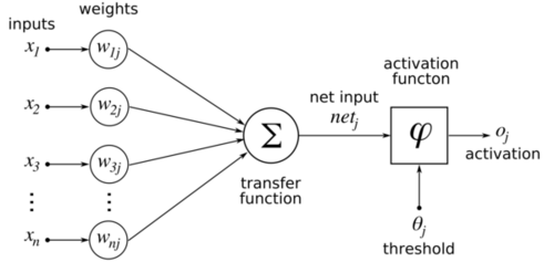
Figure 3.4 illustrates the fundamental building blocks of a perceptron, which serves as the foundation for more complex neural networks. A perceptron can be thought of as a miniature decision-maker, utilizing its weights, bias, and activation function to process inputs and generate outputs based on learned parameters. This concept forms the basis for understanding more intricate neural network architectures, such as multilayer perceptrons. In these advanced structures, layers of perceptrons work in concert, with each layer’s output serving as the input for the subsequent layer. This hierarchical arrangement creates a deep learning model capable of comprehending and modeling complex, abstract patterns within data. By stacking these simple units, neural networks gain the ability to tackle increasingly sophisticated tasks, from image recognition to natural language processing.
3.2.2 Multilayer Perceptrons
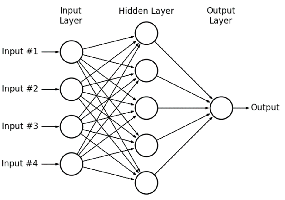
Multilayer perceptrons (MLPs) are an evolution of the single-layer perceptron model, featuring multiple layers of nodes connected in a feedforward manner. In a feedforward network, information moves in only one direction - from the input layer, through the hidden layers, to the output layer, without any cycles or loops. This structure is illustrated in Figure 3.5. The network layers include an input layer for data reception, several hidden layers for data processing, and an output layer for final result generation.
While a single perceptron is limited in its capacity to model complex patterns, the real strength of neural networks emerges from the assembly of multiple layers. Each layer consists of numerous perceptrons working together, allowing the network to capture intricate and non-linear relationships within the data. With sufficient depth and breadth, these networks can approximate virtually any function, no matter how complex.
3.2.3 Training Process
A neural network receives an input, performs a calculation, and produces a prediction. The prediction is determined by the calculations performed within the sets of perceptrons found between the input and output layers. These calculations depend primarily on the input and the weights. Since you do not have control over the input, the objective during training is to adjust the weights in such a way that the output of the network provides the most accurate prediction.
The training process involves several key steps, beginning with the forward pass, where the existing weights of the network are used to calculate the output for a given input. This output is then compared to the true target values to calculate an error, which measures how well the network’s prediction matches the expected outcome. Following this, a backward pass is performed. This involves using the error to make adjustments to the weights of the network through a process called backpropagation. This adjustment reduces the error in subsequent predictions. The cycle of forward pass, error calculation, and backward pass is repeated iteratively. This process continues until the network’s predictions are sufficiently accurate or a predefined number of iterations is reached, effectively minimizing the loss function used to measure the error.
Forward Pass
The forward pass is the initial phase where data moves through the network from the input to the output layer. At the start of training, the network’s weights are randomly initialized, setting the initial conditions for learning. During the forward pass, each layer performs specific computations on the input data using these weights and biases, and the results are then passed to the subsequent layer. The final output of this phase is the network’s prediction. This prediction is compared to the actual target values present in the dataset to calculate the loss, which can be thought of as the difference between the predicted outputs and the target values. The loss quantifies the network’s performance at this stage, providing a crucial metric for the subsequent adjustment of weights during the backward pass.
Video 3.1 below explains how neural networks work using handwritten digit recognition as an example application. It also touches on the math underlying neural nets.
Backward Pass (Backpropagation)
After completing the forward pass and computing the loss, which measures how far the model’s predictions deviate from the actual target values, the next step is to improve the model’s performance by adjusting the network’s weights. Since we cannot control the inputs to the model, adjusting the weights becomes our primary method for refining the model.
We determine how to adjust the weights of our model through a key algorithm called backpropagation. Backpropagation uses the calculated loss to determine the gradient of each weight. These gradients describe the direction and magnitude in which the weights should be adjusted. By tuning the weights based on these gradients, the model is better positioned to make predictions that are closer to the actual target values in the next forward pass.
Grasping these foundational concepts paves the way to understanding more intricate deep learning architectures and techniques, fostering the development of more sophisticated and productive applications, especially within embedded AI systems.
Video 3.2 and Video 3.3 build upon Video 3.1. They cover gradient descent and backpropagation in neural networks.
3.2.4 Model Architectures
Deep learning architectures refer to the various structured approaches that dictate how neurons and layers are organized and interact in neural networks. These architectures have evolved to tackle different problems and data types effectively. This section overviews some well-known deep learning architectures and their characteristics.
Multilayer Perceptrons (MLPs)
MLPs are basic deep learning architectures comprising three layers: an input layer, one or more hidden layers, and an output layer. These layers are fully connected, meaning each neuron in a layer is linked to every neuron in the preceding and following layers. MLPs can model intricate functions and are used in various tasks, such as regression, classification, and pattern recognition. Their capacity to learn non-linear relationships through backpropagation makes them a versatile instrument in the deep learning toolkit.
In embedded AI systems, MLPs can function as compact models for simpler tasks like sensor data analysis or basic pattern recognition, where computational resources are limited. Their ability to learn non-linear relationships with relatively less complexity makes them a suitable choice for embedded systems.
We’ve just scratched the surface of neural networks. Now, you’ll get to try and apply these concepts in practical examples. In the provided Colab notebooks, you’ll explore:
Predicting house prices: Learn how neural networks can analyze housing data to estimate property values. ![]()
Image Classification: Discover how to build a network to understand the famous MNIST handwritten digit dataset. ![]()
Real-world medical diagnosis: Use deep learning to tackle the important task of breast cancer classification. ![]()
Convolutional Neural Networks (CNNs)
CNNs are mainly used in image and video recognition tasks. This architecture consists of two main parts: the convolutional base and the fully connected layers. In the convolutional base, convolutional layers filter input data to identify features like edges, corners, and textures. Following each convolutional layer, a pooling layer can be applied to reduce the spatial dimensions of the data, thereby decreasing computational load and concentrating the extracted features. Unlike MLPs, which treat input features as flat, independent entities, CNNs maintain the spatial relationships between pixels, making them particularly effective for image and video data. The extracted features from the convolutional base are then passed into the fully connected layers, similar to those used in MLPs, which perform classification based on the features extracted by the convolution layers. CNNs have proven highly effective in image recognition, object detection, and other computer vision applications.
In embedded AI, CNNs are crucial for image and video recognition tasks, where real-time processing is often needed. They can be optimized for embedded systems using techniques like quantization and pruning to minimize memory usage and computational demands, enabling efficient object detection and facial recognition functionalities in devices with limited computational resources.
We discussed that CNNs excel at identifying image features, making them ideal for tasks like object classification. Now, you’ll get to put this knowledge into action! This Colab notebook focuses on building a CNN to classify images from the CIFAR-10 dataset, which includes objects like airplanes, cars, and animals. You’ll learn about the key differences between CIFAR-10 and the MNIST dataset we explored earlier and how these differences influence model choice. By the end of this notebook, you’ll have a grasp of CNNs for image recognition and be well on your way to becoming a TinyML expert! ![]()
Recurrent Neural Networks (RNNs)
RNNs are suitable for sequential data analysis, like time series forecasting and natural language processing. In this architecture, connections between nodes form a directed graph along a temporal sequence, allowing information to be carried across sequences through hidden state vectors. Variants of RNNs include Long Short-Term Memory (LSTM) and Gated Recurrent Units (GRU), designed to capture longer dependencies in sequence data.
These networks can be used in voice recognition systems, predictive maintenance, or IoT devices where sequential data patterns are common. Optimizations specific to embedded platforms can assist in managing their typically high computational and memory requirements.
Generative Adversarial Networks (GANs)
GANs consist of two networks, a generator and a discriminator, trained simultaneously through adversarial training (Goodfellow et al. 2020). The generator produces data that tries to mimic the real data distribution, while the discriminator distinguishes between real and generated data. GANs are widely used in image generation, style transfer, and data augmentation.
In embedded settings, GANs could be used for on-device data augmentation to improve the training of models directly on the embedded device, enabling continual learning and adaptation to new data without the need for cloud computing resources.
Autoencoders
Autoencoders are neural networks for data compression and noise reduction (Bank, Koenigstein, and Giryes 2023). They are structured to encode input data into a lower-dimensional representation and then decode it back to its original form. Variants like Variational Autoencoders (VAEs) introduce probabilistic layers that allow for generative properties, finding applications in image generation and anomaly detection.
Using autoencoders can help in efficient data transmission and storage, improving the overall performance of embedded systems with limited computational and memory resources.
Transformer Networks
Transformer networks have emerged as a powerful architecture, especially in natural language processing (Vaswani et al. 2017). These networks use self-attention mechanisms to weigh the influence of different input words on each output word, enabling parallel computation and capturing intricate patterns in data. Transformer networks have led to state-of-the-art results in tasks like language translation, summarization, and text generation.
These networks can be optimized to perform language-related tasks directly on the device. For example, transformers can be used in embedded systems for real-time translation services or voice-assisted interfaces, where latency and computational efficiency are crucial. Techniques such as model distillation can be employed to deploy these networks on embedded devices with limited resources.
These architectures serve specific purposes and excel in different domains, offering a rich toolkit for addressing diverse problems in embedded AI systems. Understanding the nuances of these architectures is crucial in designing effective and efficient deep learning models for various applications.
3.2.5 Traditional ML vs Deep Learning
Deep learning extends traditional machine learning by utilizing neural networks to discern patterns in data. In contrast, traditional machine learning relies on a set of established algorithms such as decision trees, k-nearest neighbors, and support vector machines, but does not involve neural networks. To briefly highlight the differences, Table 3.1 illustrates the contrasting characteristics between traditional ML and deep learning:
| Aspect | Traditional ML | Deep Learning |
|---|---|---|
| Data Requirements | Low to Moderate (efficient with smaller datasets) | High (requires large datasets for nuanced learning) |
| Model Complexity | Moderate (suitable for well-defined problems) | High (detects intricate patterns, suited for complex tasks) |
| Computational Resources | Low to Moderate (cost-effective, less resource-intensive) | High (demands substantial computational power and resources) |
| Deployment Speed | Fast (quicker training and deployment cycles) | Slow (prolonged training times, esp. with larger datasets) |
| Interpretability | High (clear insights into decision pathways) | Low (complex layered structures, “black box” nature) |
| Maintenance | Easier (simple to update and maintain) | Complex (requires more efforts in maintenance and updates) |
3.2.6 Choosing Traditional ML vs. DL
Data Availability and Volume
Amount of Data: Traditional machine learning algorithms, such as decision trees or Naive Bayes, are often more suitable when data availability is limited. They offer robust predictions even with smaller datasets. This is particularly true in medical diagnostics for disease prediction and customer segmentation in marketing.
Data Diversity and Quality: Traditional machine learning algorithms often work well with structured data (the input to the model is a set of features, ideally independent of each other) but may require significant preprocessing effort (i.e., feature engineering). On the other hand, deep learning takes the approach of automatically performing feature engineering as part of the model architecture. This approach enables the construction of end-to-end models capable of directly mapping from unstructured input data (such as text, audio, and images) to the desired output without relying on simplistic heuristics that have limited effectiveness. However, this results in larger models demanding more data and computational resources. In noisy data, the necessity for larger datasets is further emphasized when utilizing Deep Learning.
Complexity of the Problem
Problem Granularity: Problems that are simple to moderately complex, which may involve linear or polynomial relationships between variables, often find a better fit with traditional machine learning methods.
Hierarchical Feature Representation: Deep learning models are excellent in tasks that require hierarchical feature representation, such as image and speech recognition. However, not all problems require this complexity, and traditional machine learning algorithms may sometimes offer simpler and equally effective solutions.
Hardware and Computational Resources
Resource Constraints: The availability of computational resources often influences the choice between traditional ML and deep learning. The former is generally less resource-intensive and thus preferable in environments with hardware limitations or budget constraints.
Scalability and Speed: Traditional machine learning algorithms, like support vector machines (SVM), often allow for faster training times and easier scalability, which is particularly beneficial in projects with tight timelines and growing data volumes.
Regulatory Compliance
Regulatory compliance is crucial in various industries, requiring adherence to guidelines and best practices such as the General Data Protection Regulation (GDPR) in the EU. Traditional ML models, due to their inherent interpretability, often align better with these regulations, especially in sectors like finance and healthcare.
Interpretability
Understanding the decision-making process is easier with traditional machine learning techniques than deep learning models, which function as “black boxes,” making it challenging to trace decision pathways.
3.2.7 Making an Informed Choice
Given the constraints of embedded AI systems, understanding the differences between traditional ML techniques and deep learning becomes essential. Both avenues offer unique advantages, and their distinct characteristics often dictate the choice of one over the other in different scenarios.
Despite this, deep learning has steadily outperformed traditional machine learning methods in several key areas due to abundant data, computational advancements, and proven effectiveness in complex tasks. Here are some specific reasons why we focus on deep learning:
1. Superior Performance in Complex Tasks: Deep learning models, particularly deep neural networks, excel in tasks where the relationships between data points are incredibly intricate. Tasks like image and speech recognition, language translation, and playing complex games like Go and Chess have seen significant advancements primarily through deep learning algorithms.
2. Efficient Handling of Unstructured Data: Unlike traditional machine learning methods, deep learning can more effectively process unstructured data. This is crucial in today’s data landscape, where the vast majority of data, such as text, images, and videos, is unstructured.
3. Leveraging Big Data: With the availability of big data, deep learning models can learn and improve continually. These models excel at utilizing large datasets to improve their predictive accuracy, a limitation in traditional machine-learning approaches.
4. Hardware Advancements and Parallel Computing: The advent of powerful GPUs and the availability of cloud computing platforms have enabled the rapid training of deep learning models. These advancements have addressed one of deep learning’s significant challenges: the need for substantial computational resources.
5. Dynamic Adaptability and Continuous Learning: Deep learning models can dynamically adapt to new information or data. They can be trained to generalize their learning to new, unseen data, crucial in rapidly evolving fields like autonomous driving or real-time language translation.
While deep learning has gained significant traction, it’s essential to understand that traditional machine learning is still relevant. As we dive deeper into the intricacies of deep learning, we will also highlight situations where traditional machine learning methods may be more appropriate due to their simplicity, efficiency, and interpretability. By focusing on deep learning in this text, we aim to equip readers with the knowledge and tools to tackle modern, complex problems across various domains while also providing insights into the comparative advantages and appropriate application scenarios for deep learning and traditional machine learning techniques.
3.3 Conclusion
Deep learning has become a potent set of techniques for addressing intricate pattern recognition and prediction challenges. Starting with an overview, we outlined the fundamental concepts and principles governing deep learning, laying the groundwork for more advanced studies.
Central to deep learning, we explored the basic ideas of neural networks, powerful computational models inspired by the human brain’s interconnected neuron structure. This exploration allowed us to appreciate neural networks’ capabilities and potential in creating sophisticated algorithms capable of learning and adapting from data.
Understanding the role of libraries and frameworks was a key part of our discussion. We offered insights into the tools that can facilitate developing and deploying deep learning models. These resources ease the implementation of neural networks and open avenues for innovation and optimization.
Next, we tackled the challenges one might face when embedding deep learning algorithms within embedded systems, providing a critical perspective on the complexities and considerations of bringing AI to edge devices.
Furthermore, we examined deep learning’s limitations. Through discussions, we unraveled the challenges faced in deep learning applications and outlined scenarios where traditional machine learning might outperform deep learning. These sections are crucial for fostering a balanced view of deep learning’s capabilities and limitations.
In this primer, we have equipped you with the knowledge to make informed choices between deploying traditional machine learning or deep learning techniques, depending on the unique demands and constraints of a specific problem.
As we conclude this chapter, we hope you are now well-equipped with the basic “language” of deep learning and prepared to go deeper into the subsequent chapters with a solid understanding and critical perspective. The journey ahead is filled with exciting opportunities and challenges in embedding AI within systems.
3.4 Resources
Here is a curated list of resources to support students and instructors in their learning and teaching journeys. We are continuously working on expanding this collection and will be adding new exercises soon.
These slides are a valuable tool for instructors to deliver lectures and for students to review the material at their own pace. We encourage students and instructors to leverage these slides to improve their understanding and facilitate effective knowledge transfer.
To reinforce the concepts covered in this chapter, we have curated a set of exercises that challenge students to apply their knowledge and deepen their understanding.
- Coming soon.