8 Efficient AI
Resources: Slides, Videos, Exercises, Labs

Efficiency in artificial intelligence (AI) is not simply a luxury but a necessity. In this chapter, we dive into the key concepts underpinning AI systems’ efficiency. The computational demands on neural networks can be daunting, even for minimal systems. For AI to be seamlessly integrated into everyday devices and essential systems, it must perform optimally within the constraints of limited resources while maintaining its efficacy. The pursuit of efficiency guarantees that AI models are streamlined, rapid, and sustainable, thereby widening their applicability across various platforms and scenarios.
Recognize the need for efficient AI in TinyML/edge devices.
Understand the need for efficient model architectures like MobileNets and SqueezeNet.
Understand why techniques for model compression are important.
Gain an appreciation for the value of efficient AI hardware.
Recognize the importance of numerical representations and their precision.
Understand the nuances of model comparison beyond just accuracy.
Recognize that model comparison involves memory, computation, power, and speed, not just accuracy.
Recognize efficiency encompasses technology, costs, and ethics.
The focus is on gaining a conceptual understanding of the motivations and significance of the various strategies for achieving efficient AI, both in terms of techniques and a holistic perspective. Subsequent chapters provide a more in-depth exploration of these multiple concepts.
8.1 Introduction
Training models can consume significant energy, sometimes equivalent to the carbon footprint of sizable industrial processes. We will cover some of these sustainability details in the AI Sustainability chapter. On the deployment side, if these models are not optimized for efficiency, they can quickly drain device batteries, demand excessive memory, or fall short of real-time processing needs. Through this chapter, we aim to elucidate the nuances of efficiency, setting the groundwork for a comprehensive exploration in the subsequent chapters.
8.2 The Need for Efficient AI
Efficiency takes on different connotations depending on where AI computations occur. Let’s revisit Cloud, Edge, and TinyML (as discussed in ML Systems) and differentiate between them in terms of efficiency. Figure 8.1 provides a big-picture comparison of the three different platforms.
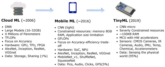
Cloud AI: Traditional AI models often run in large-scale data centers equipped with powerful GPUs and TPUs (Barroso, Hölzle, and Ranganathan 2019). Here, efficiency pertains to optimizing computational resources, reducing costs, and ensuring timely data processing and return. However, relying on the cloud introduces latency, especially when dealing with large data streams that require uploading, processing, and downloading.
Edge AI: Edge computing brings AI closer to the data source, processing information directly on local devices like smartphones, cameras, or industrial machines (Li et al. 2020). Here, efficiency encompasses quick real-time responses and reduced data transmission needs. However, the constraints are tighter—these devices, while more powerful than microcontrollers, have limited computational power compared to cloud setups.
TinyML: TinyML pushes the boundaries by enabling AI models to run on microcontrollers or extremely resource-constrained environments. The processor and memory performance difference between TinyML and cloud or mobile systems can be several orders of magnitude (Warden and Situnayake 2019). Efficiency in TinyML is about ensuring models are lightweight enough to fit on these devices, consume minimal energy (critical for battery-powered devices), and still perform their tasks effectively.
The spectrum from Cloud to TinyML represents a shift from vast, centralized computational resources to distributed, localized, and constrained environments. As we transition from one to the other, the challenges and strategies related to efficiency evolve, underlining the need for specialized approaches tailored to each scenario. Having established the need for efficient AI, especially within the context of TinyML, we will transition to exploring the methodologies devised to meet these challenges. The following sections outline the main concepts we will dive deeper into later. We will demonstrate the breadth and depth of innovation needed to achieve efficient AI as we explore these strategies.
8.3 Efficient Model Architectures
Selecting an optimal model architecture is as crucial as optimizing it. In recent years, researchers have made significant strides in exploring innovative architectures that can inherently have fewer parameters while maintaining strong performance.
MobileNets: MobileNets are efficient mobile and embedded vision application models (Howard et al. 2017). The key idea that led to their success is depth-wise separable convolutions, significantly reducing the number of parameters and computations in the network. MobileNetV2 and V3 further enhance this design by introducing inverted residuals and linear bottlenecks.
SqueezeNet: SqueezeNet is a class of ML models known for its smaller size without sacrificing accuracy. It achieves this by using a “fire module” that reduces the number of input channels to 3x3 filters, thus reducing the parameters (Iandola et al. 2016). Moreover, it employs delayed downsampling to increase the accuracy by maintaining a larger feature map.
ResNet variants: The Residual Network (ResNet) architecture allows for the introduction of skip connections or shortcuts (He et al. 2016). Some variants of ResNet are designed to be more efficient. For instance, ResNet-SE incorporates the “squeeze and excitation” mechanism to recalibrate feature maps (Hu, Shen, and Sun 2018), while ResNeXt offers grouped convolutions for efficiency (Xie et al. 2017).
8.4 Efficient Model Compression
Model compression methods are essential for bringing deep learning models to devices with limited resources. These techniques reduce models’ size, energy consumption, and computational demands without significantly losing accuracy. At a high level, the methods can be categorized into the following fundamental methods:
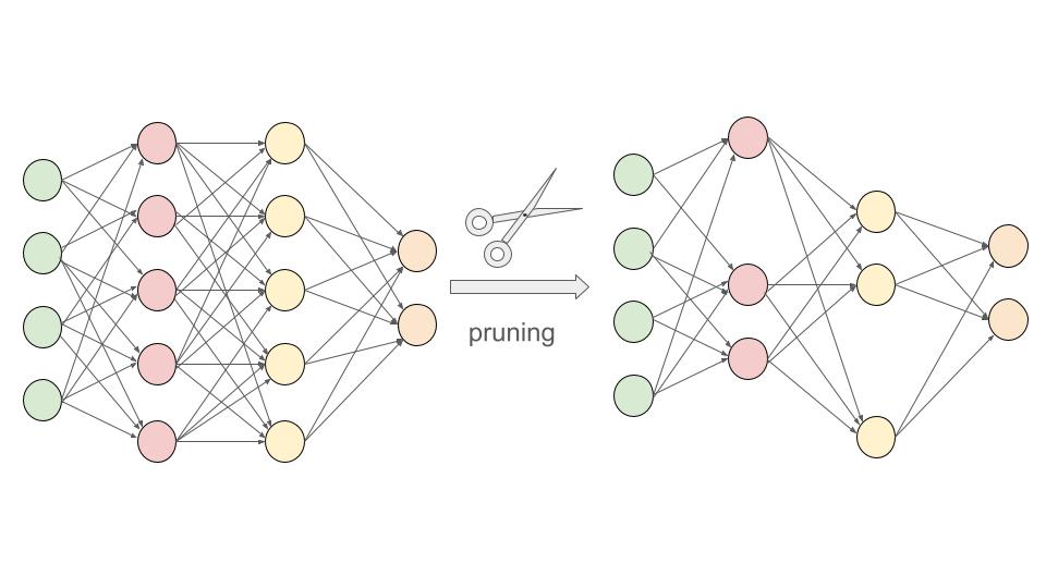
Pruning: We’ve mentioned pruning a few times in previous chapters but have not yet formally introduced it. Pruning is similar to trimming the branches of a tree. This was first thought of in the Optimal Brain Damage paper (LeCun, Denker, and Solla 1989) and was later popularized in the context of deep learning by Han, Mao, and Dally (2016). Certain weights or entire neurons are removed from the network in pruning based on specific criteria. This can significantly reduce the model size. We will explore two of the main pruning strategies, structured and unstructured pruning, in Section 9.2.1. Figure 8.2 is an example of neural network pruning, where removing some of the nodes in the inner layers (based on specific criteria) reduces the number of edges between the nodes and, in turn, the model’s size.
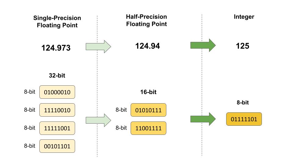
Quantization: Quantization is the process of constraining an input from a large set to output in a smaller set, primarily in deep learning; this means reducing the number of bits that represent the weights and biases of the model. For example, using 16-bit or 8-bit representations instead of 32-bit can reduce the model size and speed up computations, with a minor trade-off in accuracy. We will explore these in more detail in Section 9.3.4. Figure 8.3 shows an example of quantization by rounding to the closest number. The conversion from 32-bit floating point to 16-bit reduces memory usage by 50%. Going from a 32-bit to an 8-bit integer reduces memory usage by 75%. While the loss in numeric precision, and consequently model performance, is minor, the memory usage efficiency is significant.
Knowledge Distillation: Knowledge distillation involves training a smaller model (student) to replicate the behavior of a larger model (teacher). The idea is to transfer the knowledge from the cumbersome model to the lightweight one. Hence, the smaller model attains performance close to its larger counterpart but with significantly fewer parameters. We will explore knowledge distillation in more detail in the Section 9.2.2.1.
8.5 Efficient Inference Hardware
In the Training chapter, we discussed the process of training AI models. Now, from an efficiency standpoint, it’s important to note that training is a resource and time-intensive task, often requiring powerful hardware and taking anywhere from hours to weeks to complete. Inference, on the other hand, needs to be as fast as possible, especially in real-time applications. This is where efficient inference hardware comes into play. By optimizing the hardware specifically for inference tasks, we can achieve rapid response times and power-efficient operation, which is especially crucial for edge devices and embedded systems.
TPUs (Tensor Processing Units): TPUs are custom-built ASICs (Application-Specific Integrated Circuits) by Google to accelerate machine learning workloads (Jouppi et al. 2017). They are optimized for tensor operations, offering high throughput for low-precision arithmetic, and are designed specifically for neural network machine learning. TPUs significantly accelerate model training and inference compared to general-purpose GPU/CPUs. This boost means faster model training and real-time or near-real-time inference capabilities, crucial for applications like voice search and augmented reality.
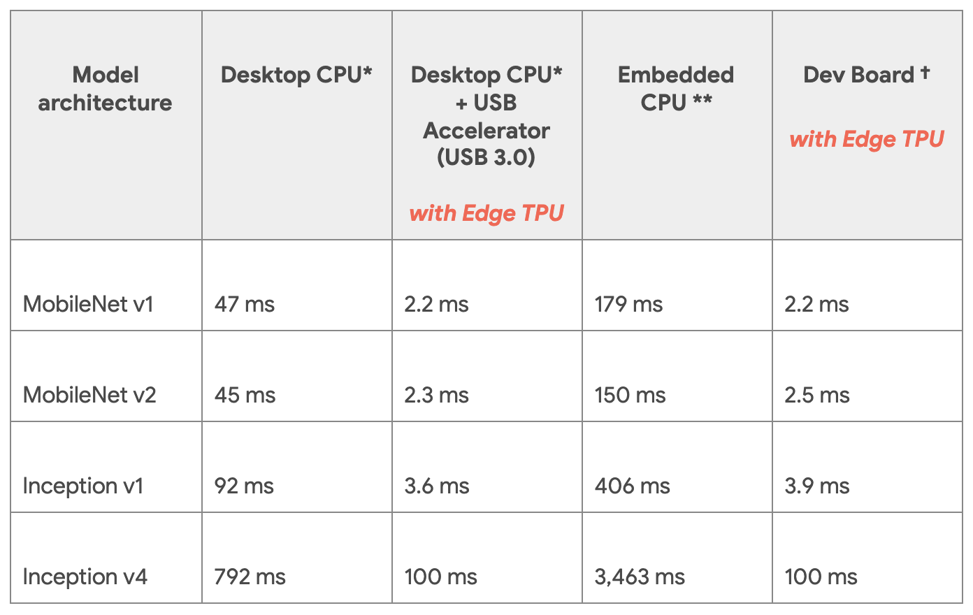
Edge TPUs are a smaller, power-efficient version of Google’s TPUs tailored for edge devices. They provide fast on-device ML inferencing for TensorFlow Lite models. Edge TPUs allow for low-latency, high-efficiency inference on edge devices like smartphones, IoT devices, and embedded systems. AI capabilities can be deployed in real-time applications without communicating with a central server, thus saving bandwidth and reducing latency. Consider the table in Figure 8.4. It shows the performance differences between running different models on CPUs versus a Coral USB accelerator. The Coral USB accelerator is an accessory by Google’s Coral AI platform that lets developers connect Edge TPUs to Linux computers. Running inference on the Edge TPUs was 70 to 100 times faster than on CPUs.
NN (Neural Network) Accelerators: Fixed-function neural network accelerators are hardware accelerators designed explicitly for neural network computations. They can be standalone chips or part of a larger system-on-chip (SoC) solution. By optimizing the hardware for the specific operations that neural networks require, such as matrix multiplications and convolutions, NN accelerators can achieve faster inference times and lower power consumption than general-purpose CPUs and GPUs. They are especially beneficial in TinyML devices with power or thermal constraints, such as smartwatches, micro-drones, or robotics.
But these are all but the most common examples. Several other types of hardware are emerging that have the potential to offer significant advantages for inference. These include, but are not limited to, neuromorphic hardware, photonic computing, etc. In Section 10.3, we will explore these in greater detail.
Efficient hardware for inference speeds up the process, saves energy, extends battery life, and can operate in real-time conditions. As AI continues to be integrated into myriad applications, from smart cameras to voice assistants, the role of optimized hardware will only become more prominent. By leveraging these specialized hardware components, developers and engineers can bring the power of AI to devices and situations that were previously unthinkable.
8.6 Efficient Numerics
Machine learning, and especially deep learning, involves enormous amounts of computation. Models can have millions to billions of parameters, often trained on vast datasets. Every operation, every multiplication or addition, demands computational resources. Therefore, the precision of the numbers used in these operations can significantly impact the computational speed, energy consumption, and memory requirements. This is where the concept of efficient numerics comes into play.
8.6.1 Numerical Formats
There are many different types of numerics. Numerics have a long history in computing systems.
Floating point: Known as a single-precision floating point, FP32 utilizes 32 bits to represent a number, incorporating its sign, exponent, and mantissa. Understanding how floating point numbers are represented under the hood is crucial for grasping the various optimizations possible in numerical computations. The sign bit determines whether the number is positive or negative, the exponent controls the range of values that can be represented, and the mantissa determines the precision of the number. The combination of these components allows floating point numbers to represent a vast range of values with varying degrees of precision.
Video 8.1 provides a comprehensive overview of these three main components - sign, exponent, and mantissa - and how they work together to represent floating point numbers.
FP32 is widely adopted in many deep learning frameworks and balances accuracy and computational requirements. It is prevalent in the training phase for many neural networks due to its sufficient precision in capturing minute details during weight updates. Also known as half-precision floating point, FP16 uses 16 bits to represent a number, including its sign, exponent, and fraction. It offers a good balance between precision and memory savings. FP16 is particularly popular in deep learning training on GPUs that support mixed-precision arithmetic, combining the speed benefits of FP16 with the precision of FP32 where needed.
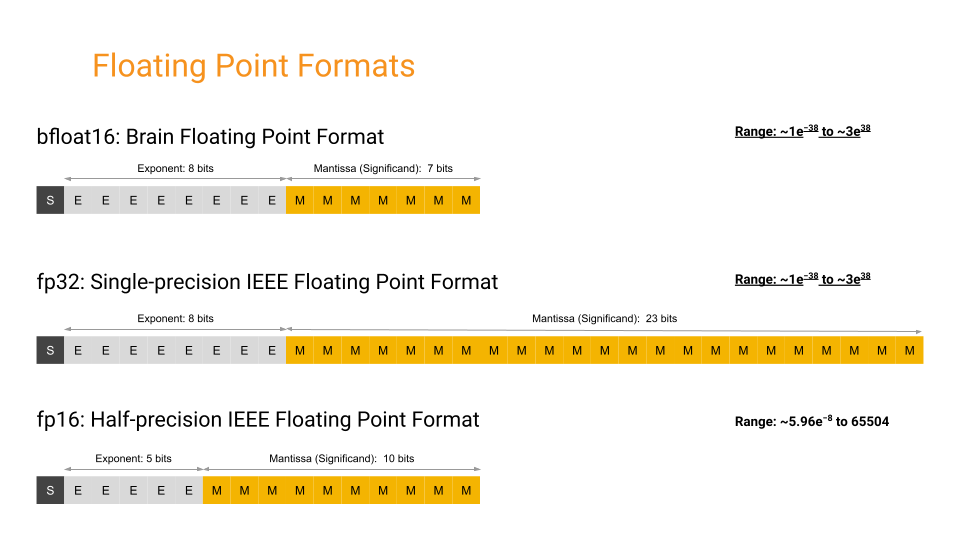
Several other numerical formats fall into an exotic class. An exotic example is BF16 or Brain Floating Point. It is a 16-bit numerical format designed explicitly for deep learning applications. It is a compromise between FP32 and FP16, retaining the 8-bit exponent from FP32 while reducing the mantissa to 7 bits (as compared to FP32’s 23-bit mantissa). This structure prioritizes range over precision. BF16 has achieved training results comparable in accuracy to FP32 while using significantly less memory and computational resources (Kalamkar et al. 2019). This makes it suitable not just for inference but also for training deep neural networks.
By retaining the 8-bit exponent of FP32, BF16 offers a similar range, which is crucial for deep learning tasks where certain operations can result in very large or very small numbers. At the same time, by truncating precision, BF16 allows for reduced memory and computational requirements compared to FP32. BF16 has emerged as a promising middle ground in the landscape of numerical formats for deep learning, providing an efficient and effective alternative to the more traditional FP32 and FP16 formats.
Figure 8.5 shows three different floating-point formats: Float32, Float16, and BFloat16.
Integer: These are integer representations using 8, 4, and 2 bits. They are often used during the inference phase of neural networks, where the weights and activations of the model are quantized to these lower precisions. Integer representations are deterministic and offer significant speed and memory advantages over floating-point representations. For many inference tasks, especially on edge devices, the slight loss in accuracy due to quantization is often acceptable, given the efficiency gains. An extreme form of integer numerics is for binary neural networks (BNNs), where weights and activations are constrained to one of two values: +1 or -1.
Variable bit widths: Beyond the standard widths, research is ongoing into extremely low bit-width numerics, even down to binary or ternary representations. Extremely low bit-width operations can offer significant speedups and further reduce power consumption. While challenges remain in maintaining model accuracy with such drastic quantization, advances continue to be made in this area.
Efficient numerics is not just about reducing the bit-width of numbers but understanding the trade-offs between accuracy and efficiency. As machine learning models become more pervasive, especially in real-world, resource-constrained environments, the focus on efficient numerics will continue to grow. By thoughtfully selecting and leveraging the appropriate numeric precision, one can achieve robust model performance while optimizing for speed, memory, and energy. Table 8.1 summarizes these trade-offs.
| Precision | Pros | Cons |
|---|---|---|
| FP32 (Floating Point 32-bit) |
|
|
| FP16 (Floating Point 16-bit) |
|
|
| INT8 (8-bit Integer) |
|
|
| INT4 (4-bit Integer) |
|
|
| Binary |
|
|
| Ternary |
|
|
8.6.2 Efficiency Benefits
Numerical efficiency matters for machine learning workloads for several reasons:
Computational Efficiency : High-precision computations (like FP32 or FP64) can be slow and resource-intensive. Reducing numeric precision can achieve faster computation times, especially on specialized hardware that supports lower precision.
Memory Efficiency: Storage requirements decrease with reduced numeric precision. For instance, FP16 requires half the memory of FP32. This is crucial when deploying models to edge devices with limited memory or working with large models.
Power Efficiency: Lower precision computations often consume less power, which is especially important for battery-operated devices.
Noise Introduction: Interestingly, the noise introduced using lower precision can sometimes act as a regularizer, helping to prevent overfitting in some models.
Hardware Acceleration: Many modern AI accelerators and GPUs are optimized for lower precision operations, leveraging the efficiency benefits of such numerics.
8.7 Evaluating Models
It’s worth noting that the actual benefits and trade-offs can vary based on the specific architecture of the neural network, the dataset, the task, and the hardware being used. Before deciding on a numeric precision, it’s advisable to perform experiments to evaluate the impact on the desired application.
8.7.1 Efficiency Metrics
A deep understanding of model evaluation methods is important to guide this process systematically. When assessing AI models’ effectiveness and suitability for various applications, efficiency metrics come to the forefront.
FLOPs (Floating Point Operations), as introduced in Training, gauge a model’s computational demands. For instance, a modern neural network like BERT has billions of FLOPs, which might be manageable on a powerful cloud server but would be taxing on a smartphone. Higher FLOPs can lead to more prolonged inference times and significant power drain, especially on devices without specialized hardware accelerators. Hence, for real-time applications such as video streaming or gaming, models with lower FLOPs might be more desirable.
Memory Usage pertains to how much storage the model requires, affecting both the deploying device’s storage and RAM. Consider deploying a model onto a smartphone: a model that occupies several gigabytes of space not only consumes precious storage but might also be slower due to the need to load large weights into memory. This becomes especially crucial for edge devices like security cameras or drones, where minimal memory footprints are vital for storage and rapid data processing.
Power Consumption becomes especially crucial for devices that rely on batteries. For instance, a wearable health monitor using a power-hungry model could drain its battery in hours, rendering it impractical for continuous health monitoring. Optimizing models for low power consumption becomes essential as we move toward an era dominated by IoT devices, where many devices operate on battery power.
Inference Time is about how swiftly a model can produce results. In applications like autonomous driving, where split-second decisions are the difference between safety and calamity, models must operate rapidly. If a self-driving car’s model takes even a few seconds too long to recognize an obstacle, the consequences could be dire. Hence, ensuring a model’s inference time aligns with the real-time demands of its application is paramount.
In essence, these efficiency metrics are more than numbers dictating where and how a model can be effectively deployed. A model might boast high accuracy, but if its FLOPs, memory usage, power consumption, or inference time make it unsuitable for its intended platform or real-world scenarios, its practical utility becomes limited.
8.7.2 Efficiency Comparisons
The landscape of machine learning models is vast, with each model offering a unique set of strengths and implementation considerations. While raw accuracy figures or training and inference speeds might be tempting benchmarks, they provide an incomplete picture. A deeper comparative analysis reveals several critical factors influencing a model’s suitability for TinyML applications. Often, we encounter the delicate balance between accuracy and efficiency. For instance, while a dense, deep learning model and a lightweight MobileNet variant might excel in image classification, their computational demands could be at two extremes. This differentiation is especially pronounced when comparing deployments on resource-abundant cloud servers versus constrained TinyML devices. In many real-world scenarios, the marginal gains in accuracy could be overshadowed by the inefficiencies of a resource-intensive model.
Moreover, the optimal model choice is not always universal but often depends on the specifics of an application. For instance, a model that excels in general object detection scenarios might struggle in niche environments, such as detecting manufacturing defects on a factory floor. This adaptability- or the lack of it- can influence a model’s real-world utility.
Another important consideration is the relationship between model complexity and its practical benefits. Take voice-activated assistants, such as “Alexa” or “OK Google.” While a complex model might demonstrate a marginally superior understanding of user speech if it’s slower to respond than a simpler counterpart, the user experience could be compromised. Thus, adding layers or parameters only sometimes equates to better real-world outcomes.
Another important consideration is the relationship between model complexity and its practical benefits. Take voice-activated assistants like “Alexa” or “OK Google.” While a complex model might demonstrate a marginally superior understanding of user speech if it’s slower to respond than a simpler counterpart, the user experience could be compromised. Thus, adding layers or parameters only sometimes equates to better real-world outcomes.
Furthermore, while benchmark datasets, such as ImageNet (Russakovsky et al. 2015), COCO (Lin et al. 2014), Visual Wake Words (Wang and Zhan 2019), Google Speech Commands (Warden 2018), etc. provide a standardized performance metric, they might not capture the diversity and unpredictability of real-world data. Two facial recognition models with similar benchmark scores might exhibit varied competencies when faced with diverse ethnic backgrounds or challenging lighting conditions. Such disparities underscore the importance of robustness and consistency across varied data. For example, Figure 8.6 from the Dollar Street dataset shows stove images across extreme monthly incomes. Stoves have different shapes and technological levels across different regions and income levels. A model that is not trained on diverse datasets might perform well on a benchmark but fail in real-world applications. So, if a model was trained on pictures of stoves found in wealthy countries only, it would fail to recognize stoves from poorer regions.

In essence, a thorough comparative analysis transcends numerical metrics. It’s a holistic assessment intertwined with real-world applications, costs, and the intricate subtleties that each model brings to the table. This is why having standard benchmarks and metrics widely established and adopted by the community becomes important.
8.8 Conclusion
Efficient AI is crucial as we push towards broader and more diverse real-world deployment of machine learning. This chapter provided an overview, exploring the various methodologies and considerations behind achieving efficient AI, starting with the fundamental need, similarities, and differences across cloud, Edge, and TinyML systems.
We examined efficient model architectures and their usefulness for optimization. Model compression techniques such as pruning, quantization, and knowledge distillation exist to help reduce computational demands and memory footprint without significantly impacting accuracy. Specialized hardware like TPUs and NN accelerators offer optimized silicon for neural network operations and data flow. Efficient numerics balance precision and efficiency, enabling models to attain robust performance using minimal resources. We will explore these topics in depth and detail in the subsequent chapters.
Together, these form a holistic framework for efficient AI. But the journey doesn’t end here. Achieving optimally efficient intelligence requires continued research and innovation. As models become more sophisticated, datasets grow, and applications diversify into specialized domains, efficiency must evolve in lockstep. Measuring real-world impact requires nuanced benchmarks and standardized metrics beyond simplistic accuracy figures.
Moreover, efficient AI expands beyond technological optimization and encompasses costs, environmental impact, and ethical considerations for the broader societal good. As AI permeates industries and daily lives, a comprehensive outlook on efficiency underpins its sustainable and responsible progress. The subsequent chapters will build upon these foundational concepts, providing actionable insights and hands-on best practices for developing and deploying efficient AI solutions.
8.9 Resources
Here is a curated list of resources to support students and instructors in their learning and teaching journeys. We are continuously working on expanding this collection and will add new exercises soon.
These slides are a valuable tool for instructors to deliver lectures and for students to review the material at their own pace. We encourage students and instructors to leverage these slides to improve their understanding and facilitate effective knowledge transfer.
- Coming soon.
To reinforce the concepts covered in this chapter, we have curated a set of exercises that challenge students to apply their knowledge and deepen their understanding.
- Coming soon.
In addition to exercises, we offer a series of hands-on labs allowing students to gain practical experience with embedded AI technologies. These labs provide step-by-step guidance, enabling students to develop their skills in a structured and supportive environment. We are excited to announce that new labs will be available soon, further enriching the learning experience.
- Coming soon.