6 AI Frameworks
Resources: Slides, Videos, Exercises, Labs

This chapter explores the landscape of AI frameworks that serve as the foundation for developing machine learning systems. AI frameworks provide the tools, libraries, and environments to design, train, and deploy machine learning models. We explore the evolutionary trajectory of these frameworks, dissect the workings of TensorFlow, and provide insights into the core components and advanced features that define these frameworks.
Furthermore, we investigate the specialization of frameworks tailored to specific needs, the emergence of frameworks specifically designed for embedded AI, and the criteria for selecting the most suitable framework for your project. This exploration will be rounded off by a glimpse into the future trends expected to shape the landscape of ML frameworks in the coming years.
Understand the evolution and capabilities of major machine learning frameworks. This includes graph execution models, programming paradigms, hardware acceleration support, and how they have expanded over time.
Learn frameworks’ core components and functionality, such as computational graphs, data pipelines, optimization algorithms, training loops, etc., that enable efficient model building.
Compare frameworks across different environments, such as cloud, edge, and TinyML. Learn how frameworks specialize based on computational constraints and hardware.
Dive deeper into embedded and TinyML-focused frameworks like TensorFlow Lite Micro, CMSIS-NN, TinyEngine, etc., and how they optimize for microcontrollers.
When choosing a framework, explore model conversion and deployment considerations, including latency, memory usage, and hardware support.
Evaluate key factors in selecting the right framework, like performance, hardware compatibility, community support, ease of use, etc., based on the specific project needs and constraints.
Understand the limitations of current frameworks and potential future trends, such as using ML to improve frameworks, decomposed ML systems, and high-performance compilers.
6.1 Introduction
Machine learning frameworks provide the tools and infrastructure to efficiently build, train, and deploy machine learning models. In this chapter, we will explore the evolution and key capabilities of major frameworks like TensorFlow (TF), PyTorch, and specialized frameworks for embedded devices. We will dive into the components like computational graphs, optimization algorithms, hardware acceleration, and more that enable developers to construct performant models quickly. Understanding these frameworks is essential to leverage the power of deep learning across the spectrum from cloud to edge devices.
ML frameworks handle much of the complexity of model development through high-level APIs and domain-specific languages that allow practitioners to quickly construct models by combining pre-made components and abstractions. For example, frameworks like TensorFlow and PyTorch provide Python APIs to define neural network architectures using layers, optimizers, datasets, and more. This enables rapid iteration compared to coding every model detail from scratch.
A key capability offered by these frameworks is distributed training engines that can scale model training across clusters of GPUs and TPUs. This makes it feasible to train state-of-the-art models with billions or trillions of parameters on vast datasets. Frameworks also integrate with specialized hardware like NVIDIA GPUs to further accelerate training via optimizations like parallelization and efficient matrix operations.
In addition, frameworks simplify deploying finished models into production through tools like TensorFlow Serving for scalable model serving and TensorFlow Lite for optimization on mobile and edge devices. Other valuable capabilities include visualization, model optimization techniques like quantization and pruning, and monitoring metrics during training.
Leading open-source frameworks like TensorFlow, PyTorch, and MXNet power much of AI research and development today. Commercial offerings like Amazon SageMaker and Microsoft Azure Machine Learning integrate these open source frameworks with proprietary capabilities and enterprise tools.
Machine learning engineers and practitioners leverage these robust frameworks to focus on high-value tasks like model architecture, feature engineering, and hyperparameter tuning instead of infrastructure. The goal is to build and deploy performant models that solve real-world problems efficiently.
In this chapter, we will explore today’s leading cloud frameworks and how they have adapted models and tools specifically for embedded and edge deployment. We will compare programming models, supported hardware, optimization capabilities, and more to fully understand how frameworks enable scalable machine learning from the cloud to the edge.
6.2 Framework Evolution
Machine learning frameworks have evolved significantly to meet the diverse needs of machine learning practitioners and advancements in AI techniques. A few decades ago, building and training machine learning models required extensive low-level coding and infrastructure. Alongside the need for low-level coding, early neural network research was constrained by insufficient data and computing power. However, machine learning frameworks have evolved considerably over the past decade to meet the expanding needs of practitioners and rapid advances in deep learning techniques. The release of large datasets like ImageNet (Deng et al. 2009) and advancements in parallel GPU computing unlocked the potential for far deeper neural networks.
The first ML frameworks, Theano by Team et al. (2016) and Caffe by Jia et al. (2014), were developed by academic institutions. Theano was created by the Montreal Institute for Learning Algorithms, while Caffe was developed by the Berkeley Vision and Learning Center. Amid growing interest in deep learning due to state-of-the-art performance of AlexNet Krizhevsky, Sutskever, and Hinton (2012) on the ImageNet dataset, private companies and individuals began developing ML frameworks, resulting in frameworks such as Keras by Chollet (2018), Chainer by Tokui et al. (2019), TensorFlow from Google (Yu et al. 2018), CNTK by Microsoft (Seide and Agarwal 2016), and PyTorch by Facebook (Ansel et al. 2024).
Many of these ML frameworks can be divided into high-level vs. low-level frameworks and static vs. dynamic computational graph frameworks. High-level frameworks provide a higher level of abstraction than low-level frameworks. High-level frameworks have pre-built functions and modules for common ML tasks, such as creating, training, and evaluating common ML models, preprocessing data, engineering features, and visualizing data, which low-level frameworks do not have. Thus, high-level frameworks may be easier to use but are less customizable than low-level frameworks (i.e., users of low-level frameworks can define custom layers, loss functions, optimization algorithms, etc.). Examples of high-level frameworks include TensorFlow/Keras and PyTorch. Examples of low-level ML frameworks include TensorFlow with low-level APIs, Theano, Caffe, Chainer, and CNTK.
Frameworks like Theano and Caffe used static computational graphs, which required defining the full model architecture upfront, thus limiting flexibility. In contract, dynamic graphs are constructed on the fly for more iterative development. Around 2016, frameworks like PyTorch and TensorFlow 2.0 began adopting dynamic graphs, providing greater flexibility for model development. We will discuss these concepts and details later in the AI Training section.
The development of these frameworks facilitated an explosion in model size and complexity over time—from early multilayer perceptrons and convolutional networks to modern transformers with billions or trillions of parameters. In 2016, ResNet models by He et al. (2016) achieved record ImageNet accuracy with over 150 layers and 25 million parameters. Then, in 2020, the GPT-3 language model from OpenAI (Brown et al. 2020) pushed parameters to an astonishing 175 billion using model parallelism in frameworks to train across thousands of GPUs and TPUs.
Each generation of frameworks unlocked new capabilities that powered advancement:
Theano and TensorFlow (2015) introduced computational graphs and automatic differentiation to simplify model building.
CNTK (2016) pioneered efficient distributed training by combining model and data parallelism.
PyTorch (2016) provided imperative programming and dynamic graphs for flexible experimentation.
TensorFlow 2.0 (2019) defaulted eager execution for intuitiveness and debugging.
TensorFlow Graphics (2020) added 3D data structures to handle point clouds and meshes.
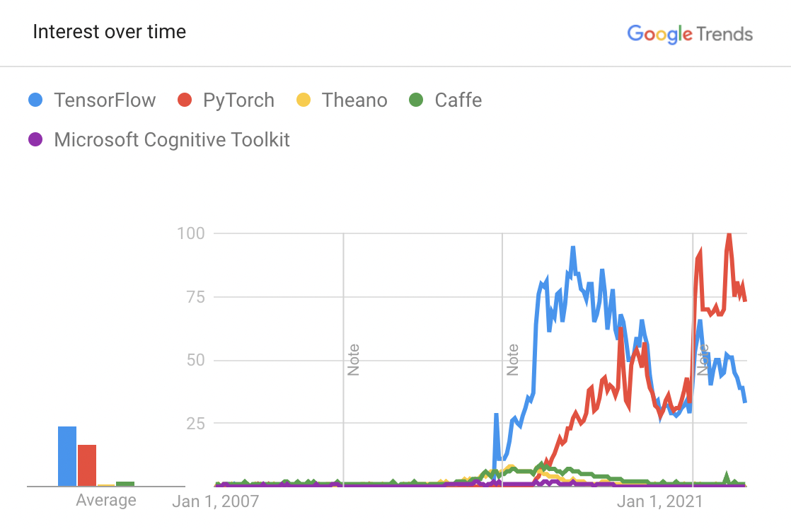
In recent years, the frameworks have converged. Figure 6.1 shows that TensorFlow and PyTorch have become the overwhelmingly dominant ML frameworks, representing more than 95% of ML frameworks used in research and production. Keras was integrated into TensorFlow in 2019; Preferred Networks transitioned Chainer to PyTorch in 2019; and Microsoft stopped actively developing CNTK in 2022 to support PyTorch on Windows.
A one-size-fits-all approach does not work well across the spectrum from cloud to tiny edge devices. Different frameworks represent various philosophies around graph execution, declarative versus imperative APIs, and more. Declaratives define what the program should do, while imperatives focus on how it should be done step-by-step. For instance, TensorFlow uses graph execution and declarative-style modeling, while PyTorch adopts eager execution and imperative modeling for more Pythonic flexibility. Each approach carries tradeoffs which we will discuss in Section 6.3.7.
Today’s advanced frameworks enable practitioners to develop and deploy increasingly complex models - a key driver of innovation in the AI field. These frameworks continue to evolve and expand their capabilities for the next generation of machine learning. To understand how these systems continue to evolve, we will dive deeper into TensorFlow as an example of how the framework grew in complexity over time.
6.3 Deep Dive into TensorFlow
TensorFlow was developed by the Google Brain team and was released as an open-source software library on November 9, 2015. It was designed for numerical computation using data flow graphs and has since become popular for a wide range of machine learning and deep learning applications.
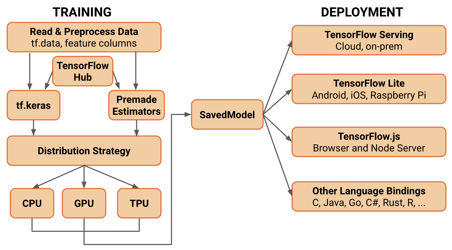
TensorFlow is a training and inference framework that provides built-in functionality to handle everything from model creation and training to deployment, as shown in Figure 6.2. Since its initial development, the TensorFlow ecosystem has grown to include many different “varieties” of TensorFlow, each intended to allow users to support ML on different platforms. In this section, we will mainly discuss only the core package.
6.3.1 TF Ecosystem
TensorFlow Core: primary package that most developers engage with. It provides a comprehensive, flexible platform for defining, training, and deploying machine learning models. It includes tf.keras as its high-level API.
TensorFlow Lite: designed for deploying lightweight models on mobile, embedded, and edge devices. It offers tools to convert TensorFlow models to a more compact format suitable for limited-resource devices and provides optimized pre-trained models for mobile.
TensorFlow Lite Micro: designed for running machine learning models on microcontrollers with minimal resources. It operates without the need for operating system support, standard C or C++ libraries, or dynamic memory allocation, using only a few kilobytes of memory.
TensorFlow.js: JavaScript library that allows training and deployment of machine learning models directly in the browser or on Node.js. It also provides tools for porting pre-trained TensorFlow models to the browser-friendly format.
TensorFlow on Edge Devices (Coral): platform of hardware components and software tools from Google that allows the execution of TensorFlow models on edge devices, leveraging Edge TPUs for acceleration.
TensorFlow Federated (TFF): framework for machine learning and other computations on decentralized data. TFF facilitates federated learning, allowing model training across many devices without centralizing the data.
TensorFlow Graphics: library for using TensorFlow to carry out graphics-related tasks, including 3D shapes and point clouds processing, using deep learning.
TensorFlow Hub: repository of reusable machine learning model components to allow developers to reuse pre-trained model components, facilitating transfer learning and model composition.
TensorFlow Serving: framework designed for serving and deploying machine learning models for inference in production environments. It provides tools for versioning and dynamically updating deployed models without service interruption.
TensorFlow Extended (TFX): end-to-end platform designed to deploy and manage machine learning pipelines in production settings. TFX encompasses data validation, preprocessing, model training, validation, and serving components.
TensorFlow was developed to address the limitations of DistBelief (Yu et al. 2018)—the framework in use at Google from 2011 to 2015—by providing flexibility along three axes: 1) defining new layers, 2) refining training algorithms, and 3) defining new training algorithms. To understand what limitations in DistBelief led to the development of TensorFlow, we will first give a brief overview of the Parameter Server Architecture that DistBelief employed (Dean et al. 2012).
The Parameter Server (PS) architecture is a popular design for distributing the training of machine learning models, especially deep neural networks, across multiple machines. The fundamental idea is to separate the storage and management of model parameters from the computation used to update these parameters. Typically, parameter servers handle the storage and management of model parameters, partitioning them across multiple servers. Worker processes perform the computational tasks, including data processing and computation of gradients, which are then sent back to the parameter servers for updating.
Storage: The stateful parameter server processes handled the storage and management of model parameters. Given the large scale of models and the system’s distributed nature, these parameters were shared across multiple parameter servers. Each server maintained a portion of the model parameters, making it "stateful" as it had to maintain and manage this state across the training process.
Computation: The worker processes, which could be run in parallel, were stateless and purely computational. They processed data and computed gradients without maintaining any state or long-term memory (M. Li et al. 2014). Workers did not retain information between different tasks. Instead, they periodically communicated with the parameter servers to retrieve the latest parameters and send back computed gradients.
Let’s comprehensively understand core machine learning algorithms using TensorFlow and their practical applications in data analysis and predictive modeling. We will start with linear regression to predict survival rates from the Titanic dataset. Then, using TensorFlow, we will construct classifiers to identify different species of flowers based on their attributes. Next, we will use the K-Means algorithm and its application in segmenting datasets into cohesive clusters. Finally, we will apply hidden Markov models (HMM) to foresee weather patterns.
![]()
Here, we will see how to build a miniature machine-learning model for microcontrollers. We will build a mini neural network that is streamlined to learn from data even with limited resources and optimized for deployment by shrinking our model for efficient use on microcontrollers. TensorFlow Lite, a powerful technology derived from TensorFlow, shrinks models for tiny devices and helps enable on-device features like image recognition in smart devices. It is used in edge computing to allow for faster analysis and decisions in devices processing data locally.
![]()
DistBelief and its architecture defined above were crucial in enabling distributed deep learning at Google but also introduced limitations that motivated the development of TensorFlow:
6.3.2 Static Computation Graph
Model parameters are distributed across various parameter servers in the parameter server architecture. Since DistBelief was primarily designed for the neural network paradigm, parameters corresponded to a fixed neural network structure. If the computation graph were dynamic, the distribution and coordination of parameters would become significantly more complicated. For example, a change in the graph might require the initialization of new parameters or the removal of existing ones, complicating the management and synchronization tasks of the parameter servers. This made it harder to implement models outside the neural framework or models that required dynamic computation graphs.
TensorFlow was designed as a more general computation framework that expresses computation as a data flow graph. This allows for a wider variety of machine learning models and algorithms outside of neural networks and provides flexibility in refining models.
6.3.3 Usability & Deployment
The parameter server model delineates roles (worker nodes and parameter servers) and is optimized for data center deployments, which might only be optimal for some use cases. For instance, this division introduces overheads or complexities on edge devices or in other non-data center environments.
TensorFlow was built to run on multiple platforms, from mobile devices and edge devices to cloud infrastructure. It also aimed to be lighter and developer-friendly and to provide ease of use between local and distributed training.
6.3.4 Architecture Design
Rather than using the parameter server architecture, TensorFlow deploys tasks across a cluster. These tasks are named processes that can communicate over a network, and each can execute TensorFlow’s core construct, the dataflow graph, and interface with various computing devices (like CPUs or GPUs). This graph is a directed representation where nodes symbolize computational operations, and edges depict the tensors (data) flowing between these operations.
Despite the absence of traditional parameter servers, some “PS tasks” still store and manage parameters reminiscent of parameter servers in other systems. The remaining tasks, which usually handle computation, data processing, and gradient calculations, are referred to as “worker tasks.” TensorFlow’s PS tasks can execute any computation representable by the dataflow graph, meaning they aren’t just limited to parameter storage, and the computation can be distributed. This capability makes them significantly more versatile and gives users the power to program the PS tasks using the standard TensorFlow interface, the same one they’d use to define their models. As mentioned above, dataflow graphs’ structure also makes them inherently good for parallelism, allowing for the processing of large datasets.
6.3.5 Built-in Functionality & Keras
TensorFlow includes libraries to help users develop and deploy more use-case-specific models, and since this framework is open-source, this list continues to grow. These libraries address the entire ML development lifecycle: data preparation, model building, deployment, and responsible AI.
One of TensorFlow’s biggest advantages is its integration with Keras, though, as we will cover in the next section, Pytorch recently added a Keras integration. Keras is another ML framework built to be extremely user-friendly and, as a result, has a high level of abstraction. We will cover Keras in more depth later in this chapter. However, when discussing its integration with TensorFlow, it was important to note that it was originally built to be backend-agnostic. This means users could abstract away these complexities, offering a cleaner, more intuitive way to define and train models without worrying about compatibility issues with different backends. TensorFlow users had some complaints about the usability and readability of TensorFlow’s API, so as TF gained prominence, it integrated Keras as its high-level API. This integration offered major benefits to TensorFlow users since it introduced more intuitive readability and portability of models while still taking advantage of powerful backend features, Google support, and infrastructure to deploy models on various platforms.
Here, we’ll learn how to use Keras, a high-level neural network API, for model development and training. We will explore the functional API for concise model building, understand loss and metric classes for model evaluation, and use built-in optimizers to update model parameters during training. Additionally, we’ll discover how to define custom layers and metrics tailored to our needs. Lastly, we’ll look into Keras’ training loops to streamline the process of training neural networks on large datasets. This knowledge will empower us to build and optimize neural network models across various machine learning and artificial intelligence applications.
![]()
6.3.6 Limitations and Challenges
TensorFlow is one of the most popular deep learning frameworks, but it has faced criticisms and weaknesses, primarily related to usability and resource usage. While advantageous, the rapid pace of updates through its support from Google has sometimes led to backward compatibility issues, deprecated functions, and shifting documentation. Additionally, even with the Keras implementation, TensorFlow’s syntax and learning curve can be difficult for new users. Another major critique of TensorFlow is its high overhead and memory consumption due to the range of built-in libraries and support. While pared-down versions can address some of these concerns, they may still be limited in resource-constrained environments.
6.3.7 PyTorch vs. TensorFlow
PyTorch and TensorFlow have established themselves as frontrunners in the industry. Both frameworks offer robust functionalities but differ in design philosophies, ease of use, ecosystem, and deployment capabilities.
Design Philosophy and Programming Paradigm: PyTorch uses a dynamic computational graph termed eager execution. This makes it intuitive and facilitates debugging since operations are executed immediately and can be inspected on the fly. In comparison, earlier versions of TensorFlow were centered around a static computational graph, which required the graph’s complete definition before execution. However, TensorFlow 2.0 introduced eager execution by default, making it more aligned with PyTorch. PyTorch’s dynamic nature and Python-based approach have enabled its simplicity and flexibility, particularly for rapid prototyping. TensorFlow’s static graph approach in its earlier versions had a steeper learning curve; the introduction of TensorFlow 2.0, with its Keras integration as the high-level API, has significantly simplified the development process.
Deployment: PyTorch is heavily favored in research environments, but deploying PyTorch models in production settings has traditionally been challenging. However, deployment has become more feasible with the introduction of TorchScript, the TorchServe tool, and PyTorch Mobile. TensorFlow stands out for its strong scalability and deployment capabilities, particularly on embedded and mobile platforms with TensorFlow Lite. TensorFlow Serving and TensorFlow.js further facilitate deployment in various environments, thus giving it a broader reach in the ecosystem.
Performance: Both frameworks offer efficient hardware acceleration for their operations. However, TensorFlow has a slightly more robust optimization workflow, such as the XLA (Accelerated Linear Algebra) compiler, which can further boost performance. Its static computational graph was also advantageous for certain optimizations in the early versions.
Ecosystem: PyTorch has a growing ecosystem with tools like TorchServe for serving models and libraries like TorchVision, TorchText, and TorchAudio for specific domains. As we mentioned earlier, TensorFlow has a broad and mature ecosystem. TensorFlow Extended (TFX) provides an end-to-end platform for deploying production machine learning pipelines. Other tools and libraries include TensorFlow Lite, TensorFlow Lite Micro, TensorFlow.js, TensorFlow Hub, and TensorFlow Serving.
Table 6.1 provides a comparative analysis:
| Aspect | Pytorch | TensorFlow |
|---|---|---|
| Design Philosophy | Dynamic computational graph (eager execution) | Static computational graph (early versions); Eager execution in TensorFlow 2.0 |
| Deployment | Traditionally challenging; Improved with TorchScript & TorchServe | Scalable, especially on embedded platforms with TensorFlow Lite |
| Performance & Optimization | Efficient GPU acceleration | Robust optimization with XLA compiler |
| Ecosystem | TorchServe, TorchVision, TorchText, TorchAudio, PyTorch Mobile | TensorFlow Extended (TFX), TensorFlow Lite, TensorFlow Lite Micro TensorFlow.js, TensorFlow Hub, TensorFlow Serving |
| Ease of Use | Preferred for its Pythonic approach and rapid prototyping | Initially steep learning curve; Simplified with Keras in TensorFlow 2.0 |
6.4 Basic Framework Components
Having introduced the popular machine learning frameworks and provided a high-level comparison, this section will introduce you to the core functionalities that form the fabric of these frameworks. It will cover the special structure called tensors, which these frameworks use to handle complex multi-dimensional data more easily. You will also learn how these frameworks represent different types of neural network architectures and their required operations through computational graphs. Additionally, you will see how they offer tools that make the development of machine learning models more abstract and efficient, such as data loaders, implemented loss optimization algorithms, efficient differentiation techniques, and the ability to accelerate your training process on hardware accelerators.
6.4.1 Tensor data structures
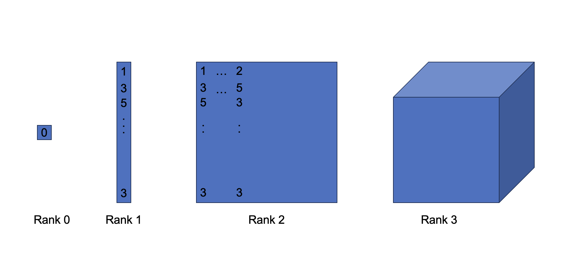
To understand tensors, let us start from the familiar concepts in linear algebra. As demonstrated in Figure 6.4, vectors can be represented as a stack of numbers in a 1-dimensional array. Matrices follow the same idea, and one can think of them as many vectors stacked on each other, making them 2 dimensional. Higher dimensional tensors work the same way. A 3-dimensional tensor is simply a set of matrices stacked on each other in another direction. Therefore, vectors and matrices can be considered special cases of tensors with 1D and 2D dimensions, respectively.
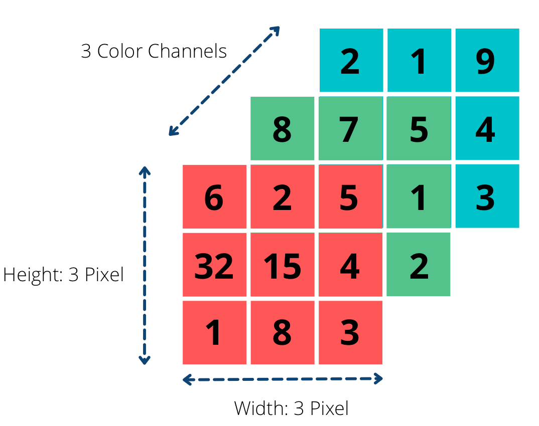
Tensors offer a flexible structure that can represent data in higher dimensions. For instance, to represent image data, the pixels at each position of an image are structured as matrices. However, images are not represented by just one matrix of pixel values; they typically have three channels where each channel is a matrix containing pixel values that represent the intensity of red, green, or blue. Together, these channels create a colored image. Without tensors, storing all this information from multiple matrices can be complex. With tensors, it is easy to contain image data in a single 3-dimensional tensor, with each number representing a certain color value at a specific location in the image.
You don’t have to stop there. If we wanted to store a series of images, we could use a 4-dimensional tensor, where the new dimension represents different images. This means you are storing multiple images, each having three matrices that represent the three color channels. This gives you an idea of the usefulness of tensors when dealing with multi-dimensional data efficiently.
Tensors also have a unique attribute that enables frameworks to automatically compute gradients, simplifying the implementation of complex models and optimization algorithms. In machine learning, as discussed in Chapter 3, backpropagation requires taking the derivative of equations. One of the key features of tensors in PyTorch and TensorFlow is their ability to track computations and calculate gradients. This is crucial for backpropagation in neural networks. For example, in PyTorch, you can use the requires_grad attribute, which allows you to automatically compute and store gradients during the backward pass, facilitating the optimization process. Similarly, in TensorFlow, tf.GradientTape records operations for automatic differentiation.
Consider this simple mathematical equation that you want to differentiate. Mathematically, you can compute the gradient in the following way:
Given: \[ y = x^2 \]
The derivative of \(y\) with respect to \(x\) is: \[ \frac{dy}{dx} = 2x \]
When \(x = 2\): \[ \frac{dy}{dx} = 2*2 = 4 \]
The gradient of \(y\) with respect to \(x\), at \(x = 2\), is 4.
A powerful feature of tensors in PyTorch and TensorFlow is their ability to easily compute derivatives (gradients). Here are the corresponding code examples in PyTorch and TensorFlow:
import torch

# Create a tensor with gradient tracking
x = torch.tensor(2.0, requires_grad=True)

# Define a simple function
y = x ** 2

# Compute the gradient
y.backward()

# Print the gradient
print(x.grad)

# Output
tensor(4.0)
import tensorflow as tf
# Create a tensor with gradient tracking
x = tf.Variable(2.0)
# Define a simple function
with tf.GradientTape() as tape:
y = x ** 2
# Compute the gradient
grad = tape.gradient(y, x)
# Print the gradient
print(grad)
# Output
tf.Tensor(4.0, shape=(), dtype=float32)This automatic differentiation is a powerful feature of tensors in frameworks like PyTorch and TensorFlow, making it easier to implement and optimize complex machine learning models.
6.4.2 Computational graphs
Graph Definition
Computational graphs are a key component of deep learning frameworks like TensorFlow and PyTorch. They allow us to express complex neural network architectures efficiently and differently. A computational graph consists of a directed acyclic graph (DAG) where each node represents an operation or variable, and edges represent data dependencies between them.
It’s important to differentiate computational graphs from neural network diagrams, such as those for multilayer perceptrons (MLPs), which depict nodes and layers. Neural network diagrams, as depicted in Chapter 3, visualize the architecture and flow of data through nodes and layers, providing an intuitive understanding of the model’s structure. In contrast, computational graphs provide a low-level representation of the underlying mathematical operations and data dependencies required to implement and train these networks.
For example, a node might represent a matrix multiplication operation, taking two input matrices (or tensors) and producing an output matrix (or tensor). To visualize this, consider the simple example in Figure 7.3. The directed acyclic graph above computes \(z = x \times y\), where each variable is just numbers.
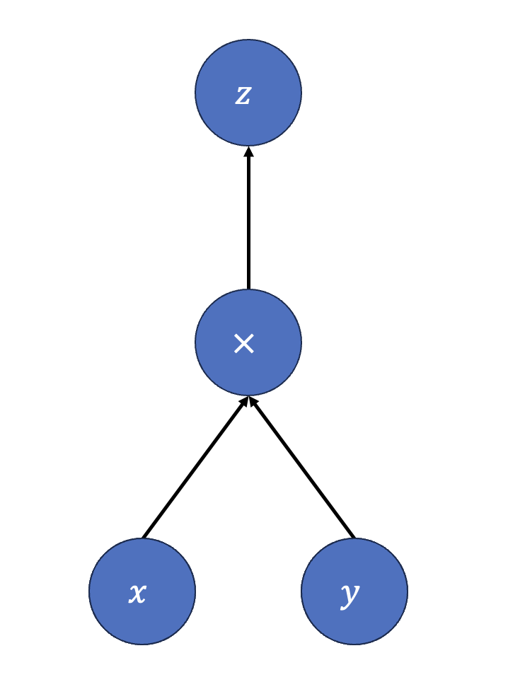
Frameworks like TensorFlow and PyTorch create computational graphs to implement the architectures of neural networks that we typically represent with diagrams. When you define a neural network layer in code (e.g., a dense layer in TensorFlow), the framework constructs a computational graph that includes all the necessary operations (such as matrix multiplication, addition, and activation functions) and their data dependencies. This graph enables the framework to efficiently manage the flow of data, optimize the execution of operations, and automatically compute gradients for training. Underneath the hood, the computational graphs represent abstractions for common layers like convolutional, pooling, recurrent, and dense layers, with data including activations, weights, and biases represented in tensors. This representation allows for efficient computation, leveraging the structure of the graph to parallelize operations and apply optimizations.
Some common layers that computational graphs might implement include convolutional layers, attention layers, recurrent layers, and dense layers. Layers serve as higher-level abstractions that define specific computations on top of the basic operations represented in the graph. For example, a Dense layer performs matrix multiplication and addition between input, weight, and bias tensors. It is important to note that a layer operates on tensors as inputs and outputs; the layer itself is not a tensor. Some key differences between layers and tensors are:
Layers contain states like weights and biases. Tensors are stateless, just holding data.
Layers can modify internal state during training. Tensors are immutable/read-only.
Layers are higher-level abstractions. Tensors are at a lower level and directly represent data and math operations.
Layers define fixed computation patterns. Tensors flow between layers during execution.
Layers are used indirectly when building models. Tensors flow between layers during execution.
So, while tensors are a core data structure that layers consume and produce, layers have additional functionality for defining parameterized operations and training. While a layer configures tensor operations under the hood, the layer remains distinct from the tensor objects. The layer abstraction makes building and training neural networks much more intuitive. This abstraction enables developers to build models by stacking these layers together without implementing the layer logic. For example, calling tf.keras.layers.Conv2D in TensorFlow creates a convolutional layer. The framework handles computing the convolutions, managing parameters, etc. This simplifies model development, allowing developers to focus on architecture rather than low-level implementations. Layer abstractions use highly optimized implementations for performance. They also enable portability, as the same architecture can run on different hardware backends like GPUs and TPUs.
In addition, computational graphs include activation functions like ReLU, sigmoid, and tanh that are essential to neural networks, and many frameworks provide these as standard abstractions. These functions introduce non-linearities that enable models to approximate complex functions. Frameworks provide these as simple, predefined operations that can be used when constructing models, for example, if.nn.relu in TensorFlow. This abstraction enables flexibility, as developers can easily swap activation functions for tuning performance. Predefined activations are also optimized by the framework for faster execution.
In recent years, models like ResNets and MobileNets have emerged as popular architectures, with current frameworks pre-packaging these as computational graphs. Rather than worrying about the fine details, developers can use them as a starting point, customizing as needed by substituting layers. This simplifies and speeds up model development, avoiding reinventing architectures from scratch. Predefined models include well-tested, optimized implementations that ensure good performance. Their modular design also enables transferring learned features to new tasks via transfer learning. These predefined architectures provide high-performance building blocks to create robust models quickly.
These layer abstractions, activation functions, and predefined architectures the frameworks provide constitute a computational graph. When a user defines a layer in a framework (e.g., tf.keras.layers.Dense()), the framework configures computational graph nodes and edges to represent that layer. The layer parameters like weights and biases become variables in the graph. The layer computations become operation nodes (such as the x and y in the figure above). When you call an activation function like tf.nn.relu(), the framework adds a ReLU operation node to the graph. Predefined architectures are just pre-configured subgraphs that can be inserted into your model’s graph. Thus, model definition via high-level abstractions creates a computational graph—the layers, activations, and architectures we use become graph nodes and edges.
We implicitly construct a computational graph when defining a neural network architecture in a framework. The framework uses this graph to determine operations to run during training and inference. Computational graphs bring several advantages over raw code, and that’s one of the core functionalities that is offered by a good ML framework:
Explicit representation of data flow and operations
Ability to optimize graph before execution
Automatic differentiation for training
Language agnosticism - graph can be translated to run on GPUs, TPUs, etc.
Portability - graph can be serialized, saved, and restored later
Computational graphs are the fundamental building blocks of ML frameworks. Model definition via high-level abstractions creates a computational graph—the layers, activations, and architectures we use become graph nodes and edges. The framework compilers and optimizers operate on this graph to generate executable code. The abstractions provide a developer-friendly API for building computational graphs. Under the hood, it’s still graphs down! So, while you may not directly manipulate graphs as a framework user, they enable your high-level model specifications to be efficiently executed. The abstractions simplify model-building, while computational graphs make it possible.
Static vs. Dynamic Graphs
Deep learning frameworks have traditionally followed one of two approaches for expressing computational graphs.
Static graphs (declare-then-execute): With this model, the entire computational graph must be defined upfront before running it. All operations and data dependencies must be specified during the declaration phase. TensorFlow originally followed this static approach - models were defined in a separate context, and then a session was created to run them. The benefit of static graphs is they allow more aggressive optimization since the framework can see the full graph. However, it also tends to be less flexible for research and interactivity. Changes to the graph require re-declaring the full model.
For example:
x = tf.placeholder(tf.float32)
y = tf.matmul(x, weights) + biases
In this example, x is a placeholder for input data, and y is the result of a matrix multiplication operation followed by an addition. The model is defined in this declaration phase, where all operations and variables must be specified upfront.
Once the entire graph is defined, the framework compiles and optimizes it. This means that the computational steps are set in stone, and the framework can apply various optimizations to improve efficiency and performance. When you later execute the graph, you provide the actual input tensors, and the pre-defined operations are carried out in the optimized sequence.
This approach is similar to building a blueprint where every detail is planned before construction begins. While this allows for powerful optimizations, it also means that any changes to the model require redefining the entire graph from scratch.
Dynamic graphs (define-by-run): Unlike declaring (all) first and then executing, the graph is built dynamically as execution happens. There is no separate declaration phase - operations execute immediately as defined. This style is imperative and flexible, facilitating experimentation.
PyTorch uses dynamic graphs, building the graph on the fly as execution happens. For example, consider the following code snippet, where the graph is built as the execution is taking place:
x = torch.randn(4,784)
y = torch.matmul(x, weights) + biases
The above example does not have separate compile/build/run phases. Ops define and execute immediately. With dynamic graphs, the definition is intertwined with execution, providing a more intuitive, interactive workflow. However, the downside is that there is less potential for optimization since the framework only sees the graph as it is built.
Recently, the distinction has blurred as frameworks adopt both modes. TensorFlow 2.0 defaults to dynamic graph mode while letting users work with static graphs when needed. Dynamic declaration offers flexibility and ease of use, making frameworks more user-friendly, while static graphs provide optimization benefits at the cost of interactivity. The ideal framework balances these approaches. Table 6.2 compares the pros and cons of static versus dynamic execution graphs:
| Execution Graph | Pros | Cons |
|---|---|---|
| Static (Declare-then-execute) |
|
|
| Dynamic (Define-by-run) |
|
|
6.4.3 Data Pipeline Tools
Computational graphs can only be as good as the data they learn from and work on. Therefore, feeding training data efficiently is crucial for optimizing deep neural network performance, though it is often overlooked as one of the core functionalities. Many modern AI frameworks provide specialized pipelines to ingest, process, and augment datasets for model training.
Data Loaders
At the core of these pipelines are data loaders, which handle reading training examples from sources like files, databases, and object storage. Data loaders facilitate efficient data loading and preprocessing, crucial for deep learning models. For instance, TensorFlow’s tf.data dataloading pipeline is designed to manage this process. Depending on the application, deep learning models require diverse data formats such as CSV files or image folders. Some popular formats include:
CSV, a versatile, simple format often used for tabular data.
TFRecord: TensorFlow’s proprietary format, optimized for performance.
Parquet: Columnar storage, offering efficient data compression and retrieval.
JPEG/PNG: Commonly used for image data.
WAV/MP3: Prevalent formats for audio data.
Data loaders batch examples to leverage vectorization support in hardware. Batching refers to grouping multiple data points for simultaneous processing, leveraging the vectorized computation capabilities of hardware like GPUs. While typical batch sizes range from 32 to 512 examples, the optimal size often depends on the data’s memory footprint and the specific hardware constraints. Advanced loaders can stream virtually unlimited datasets from disk and cloud storage. They stream large datasets from disks or networks instead of fully loading them into memory, enabling unlimited dataset sizes.
Data loaders can also shuffle data across epochs for randomization and preprocess features in parallel with model training to expedite the training process. Randomly shuffling the order of examples between training epochs reduces bias and improves generalization.
Data loaders also support caching and prefetching strategies to optimize data delivery for fast, smooth model training. Caching preprocessed batches in memory allows them to be reused efficiently during multiple training steps and eliminates redundant processing. Prefetching, conversely, involves preloading subsequent batches, ensuring that the model never idles waiting for data.
6.4.4 Data Augmentation
Machine learning frameworks like TensorFlow and PyTorch provide tools to simplify and streamline the process of data augmentation, enhancing the efficiency of expanding datasets synthetically. These frameworks offer integrated functionalities to apply random transformations, such as flipping, cropping, rotating, altering color, and adding noise for images. For audio data, common augmentations involve mixing clips with background noise or modulating speed, pitch, and volume.
By integrating augmentation tools into the data pipeline, frameworks enable these transformations to be applied on the fly during each training epoch. This approach increases the variation in the training data distribution, thereby reducing overfitting and improving model generalization. The use of performant data loaders in combination with extensive augmentation capabilities allows practitioners to efficiently feed massive, varied datasets to neural networks.
These hands-off data pipelines represent a significant improvement in usability and productivity. They allow developers to focus more on model architecture and less on data wrangling when training deep learning models.
6.4.5 Loss Functions and Optimization Algorithms
Training a neural network is fundamentally an iterative process that seeks to minimize a loss function. The goal is to fine-tune the model weights and parameters to produce predictions close to the true target labels. Machine learning frameworks have greatly streamlined this process by offering loss functions and optimization algorithms.
Machine learning frameworks provide implemented loss functions that are needed for quantifying the difference between the model’s predictions and the true values. Different datasets require a different loss function to perform properly, as the loss function tells the computer the “objective” for it to aim. Commonly used loss functions include Mean Squared Error (MSE) for regression tasks, Cross-Entropy Loss for classification tasks, and Kullback-Leibler (KL) Divergence for probabilistic models. For instance, TensorFlow’s tf.keras.losses holds a suite of these commonly used loss functions.
Optimization algorithms are used to efficiently find the set of model parameters that minimize the loss function, ensuring the model performs well on training data and generalizes to new data. Modern frameworks come equipped with efficient implementations of several optimization algorithms, many of which are variants of gradient descent with stochastic methods and adaptive learning rates. Some examples of these variants are Stochastic Gradient Descent, Adagrad, Adadelta, and Adam. The implementation of such variants are provided in tf.keras.optimizers. More information with clear examples can be found in the AI Training section.
6.4.6 Model Training Support
A compilation step is required before training a defined neural network model. During this step, the neural network’s high-level architecture is transformed into an optimized, executable format. This process comprises several steps. The first step is to construct the computational graph, which represents all the mathematical operations and data flow within the model. We discussed this earlier.
During training, the focus is on executing the computational graph. Every parameter within the graph, such as weights and biases, is assigned an initial value. Depending on the chosen initialization method, this value might be random or based on a predefined logic.
The next critical step is memory allocation. Essential memory is reserved for the model’s operations on both CPUs and GPUs, ensuring efficient data processing. The model’s operations are then mapped to the available hardware resources, particularly GPUs or TPUs, to expedite computation. Once the compilation is finalized, the model is prepared for training.
The training process employs various tools to improve efficiency. Batch processing is commonly used to maximize computational throughput. Techniques like vectorization enable operations on entire data arrays rather than proceeding element-wise, which bolsters speed. Optimizations such as kernel fusion (refer to the Optimizations chapter) amalgamate multiple operations into a single action, minimizing computational overhead. Operations can also be segmented into phases, facilitating the concurrent processing of different mini-batches at various stages.
Frameworks consistently checkpoint the state, preserving intermediate model versions during training. This ensures that progress is recovered if an interruption occurs, and training can be recommenced from the last checkpoint. Additionally, the system vigilantly monitors the model’s performance against a validation data set. Should the model begin to overfit (if its performance on the validation set declines), training is automatically halted, conserving computational resources and time.
ML frameworks incorporate a blend of model compilation, enhanced batch processing methods, and utilities such as checkpointing and early stopping. These resources manage the complex aspects of performance, enabling practitioners to zero in on model development and training. As a result, developers experience both speed and ease when utilizing neural networks’ capabilities.
6.4.7 Validation and Analysis
After training deep learning models, frameworks provide utilities to evaluate performance and gain insights into the models’ workings. These tools enable disciplined experimentation and debugging.
Evaluation Metrics
Frameworks include implementations of common evaluation metrics for validation:
Accuracy - Fraction of correct predictions overall. They are widely used for classification.
Precision - Of positive predictions, how many were positive. Useful for imbalanced datasets.
Recall - Of actual positives, how many did we predict correctly? Measures completeness.
F1-score - Harmonic mean of precision and recall. Combines both metrics.
AUC-ROC - Area under ROC curve. They are used for classification threshold analysis.
MAP - Mean Average Precision. Evaluate ranked predictions in retrieval/detection.
Confusion Matrix - Matrix that shows the true positives, true negatives, false positives, and false negatives. Provides a more detailed view of classification performance.
These metrics quantify model performance on validation data for comparison.
Visualization
Visualization tools provide insight into models:
Loss curves - Plot training and validation loss over time to spot Overfitting.
Activation grids - Illustrate features learned by convolutional filters.
Projection - Reduce dimensionality for intuitive visualization.
Precision-recall curves - Assess classification tradeoffs.
Tools like TensorBoard for TensorFlow and TensorWatch for PyTorch enable real-time metrics and visualization during training.
6.4.8 Differentiable programming
Machine learning training methods such as backpropagation rely on the change in the loss function with respect to the change in weights (which essentially is the definition of derivatives). Thus, the ability to quickly and efficiently train large machine learning models relies on the computer’s ability to take derivatives. This makes differentiable programming one of the most important elements of a machine learning framework.
We can use four primary methods to make computers take derivatives. First, we can manually figure out the derivatives by hand and input them into the computer. This would quickly become a nightmare with many layers of neural networks if we had to compute all the derivatives in the backpropagation steps by hand. Another method is symbolic differentiation using computer algebra systems such as Mathematica, which can introduce a layer of inefficiency, as there needs to be a level of abstraction to take derivatives. Numerical derivatives, the practice of approximating gradients using finite difference methods, suffer from many problems, including high computational costs and larger grid sizes, leading to many errors. This leads to automatic differentiation, which exploits the primitive functions that computers use to represent operations to obtain an exact derivative. With automatic differentiation, the computational complexity of computing the gradient is proportional to computing the function itself. Intricacies of automatic differentiation are not dealt with by end users now, but resources to learn more can be found widely, such as from here. Today’s automatic differentiation and differentiable programming are ubiquitous and are done efficiently and automatically by modern machine learning frameworks.
6.4.9 Hardware Acceleration
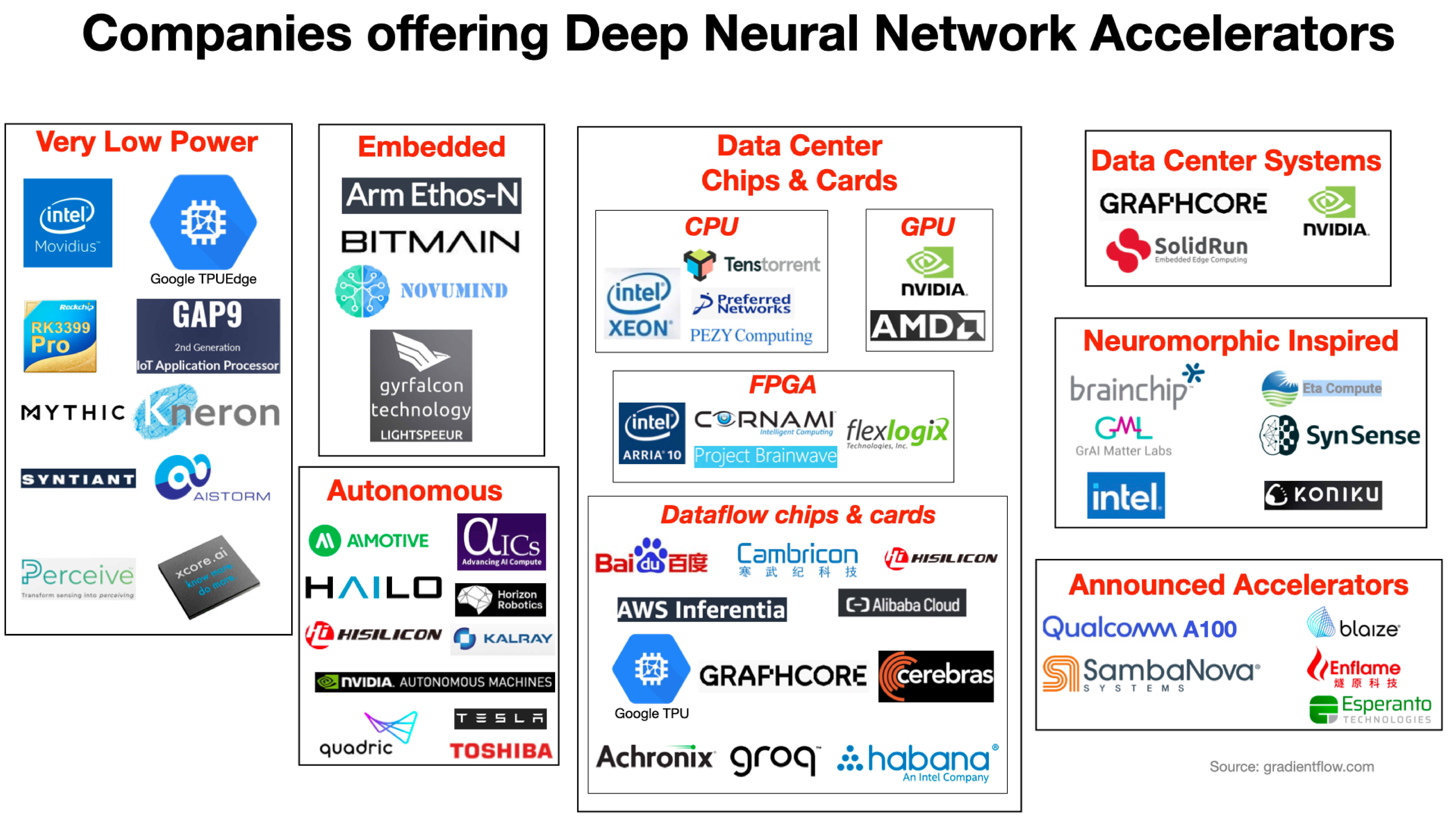
The trend to continuously train and deploy larger machine-learning models has made hardware acceleration support necessary for machine-learning platforms. Figure 6.6 shows the large number of companies that are offering hardware accelerators in different domains, such as “Very Low Power” and “Embedded” machine learning. Deep layers of neural networks require many matrix multiplications, which attract hardware that can compute matrix operations quickly and in parallel. In this landscape, two hardware architectures, the GPU and TPU, have emerged as leading choices for training machine learning models.
The use of hardware accelerators began with AlexNet, which paved the way for future works to use GPUs as hardware accelerators for training computer vision models. GPUs, or Graphics Processing Units, excel in handling many computations at once, making them ideal for the matrix operations central to neural network training. Their architecture, designed for rendering graphics, is perfect for the mathematical operations required in machine learning. While they are very useful for machine learning tasks and have been implemented in many hardware platforms, GPUs are still general purpose in that they can be used for other applications.
On the other hand, Tensor Processing Units (TPU) are hardware units designed specifically for neural networks. They focus on the multiply and accumulate (MAC) operation, and their hardware consists of a large hardware matrix that contains elements that efficiently compute the MAC operation. This concept, called the systolic array architecture, was pioneered by Kung and Leiserson (1979), but has proven to be a useful structure to efficiently compute matrix products and other operations within neural networks (such as convolutions).
While TPUs can drastically reduce training times, they also have disadvantages. For example, many operations within the machine learning frameworks (primarily TensorFlow here since the TPU directly integrates with it) are not supported by TPUs. They cannot also support custom operations from the machine learning frameworks, and the network design must closely align with the hardware capabilities.
Today, NVIDIA GPUs dominate training, aided by software libraries like CUDA, cuDNN, and TensorRT. Frameworks also include optimizations to maximize performance on these hardware types, such as pruning unimportant connections and fusing layers. Combining these techniques with hardware acceleration provides greater efficiency. For inference, hardware is increasingly moving towards optimized ASICs and SoCs. Google’s TPUs accelerate models in data centers, while Apple, Qualcomm, the NVIDIA Jetson family, and others now produce AI-focused mobile chips.
6.5 Advanced Features
Beyond providing the essential tools for training machine learning models, frameworks also offer advanced features. These features include distributing training across different hardware platforms, fine-tuning large pre-trained models with ease, and facilitating federated learning. Implementing these capabilities independently would be highly complex and resource-intensive, but frameworks simplify these processes, making advanced machine learning techniques more accessible.
6.5.1 Distributed training
As machine learning models have become larger over the years, it has become essential for large models to use multiple computing nodes in the training process. This process, distributed learning, has allowed for higher training capabilities but has also imposed challenges in implementation.
We can consider three different ways to spread the work of training machine learning models to multiple computing nodes. Input data partitioning (or data parallelism) refers to multiple processors running the same model on different input partitions. This is the easiest implementation and is available for many machine learning frameworks. The more challenging distribution of work comes with model parallelism, which refers to multiple computing nodes working on different parts of the model, and pipelined model parallelism, which refers to multiple computing nodes working on different layers of the model on the same input. The latter two mentioned here are active research areas.
ML frameworks that support distributed learning include TensorFlow (through its tf.distribute module), PyTorch (through its torch.nn.DataParallel and torch.nn.DistributedDataParallel modules), and MXNet (through its gluon API).
6.5.2 Model Conversion
Machine learning models have various methods to be represented and used within different frameworks and for different device types. For example, a model can be converted to be compatible with inference frameworks within the mobile device. The default format for TensorFlow models is checkpoint files containing weights and architectures, which are needed to retrain the models. However, models are typically converted to TensorFlow Lite format for mobile deployment. TensorFlow Lite uses a compact flat buffer representation and optimizations for fast inference on mobile hardware, discarding all the unnecessary baggage associated with training metadata, such as checkpoint file structures.
Model optimizations like quantization (see Optimizations chapter) can further optimize models for target architectures like mobile. This reduces the precision of weights and activations to uint8 or int8 for a smaller footprint and faster execution with supported hardware accelerators. For post-training quantization, TensorFlow’s converter handles analysis and conversion automatically.
Frameworks like TensorFlow simplify deploying trained models to mobile and embedded IoT devices through easy conversion APIs for TFLite format and quantization. Ready-to-use conversion enables high-performance inference on mobile without a manual optimization burden. Besides TFLite, other common targets include TensorFlow.js for web deployment, TensorFlow Serving for cloud services, and TensorFlow Hub for transfer learning. TensorFlow’s conversion utilities handle these scenarios to streamline end-to-end workflows.
More information about model conversion in TensorFlow is linked here.
6.5.3 AutoML, No-Code/Low-Code ML
In many cases, machine learning can have a relatively high barrier of entry compared to other fields. To successfully train and deploy models, one needs to have a critical understanding of a variety of disciplines, from data science (data processing, data cleaning), model structures (hyperparameter tuning, neural network architecture), hardware (acceleration, parallel processing), and more depending on the problem at hand. The complexity of these problems has led to the introduction of frameworks such as AutoML, which tries to make “Machine learning available for non-Machine Learning experts” and to “automate research in machine learning.” They have constructed AutoWEKA, which aids in the complex process of hyperparameter selection, and Auto-sklearn and Auto-pytorch, an extension of AutoWEKA into the popular sklearn and PyTorch Libraries.
While these efforts to automate parts of machine learning tasks are underway, others have focused on making machine learning models easier by deploying no-code/low-code machine learning, utilizing a drag-and-drop interface with an easy-to-navigate user interface. Companies such as Apple, Google, and Amazon have already created these easy-to-use platforms to allow users to construct machine learning models that can integrate into their ecosystem.
These steps to remove barriers to entry continue to democratize machine learning, make it easier for beginners to access, and simplify workflow for experts.
6.5.4 Advanced Learning Methods
Transfer Learning
Transfer learning is the practice of using knowledge gained from a pre-trained model to train and improve the performance of a model for a different task. For example, models such as MobileNet and ResNet are trained on the ImageNet dataset. To do so, one may freeze the pre-trained model, utilizing it as a feature extractor to train a much smaller model built on top of the feature extraction. One can also fine-tune the entire model to fit the new task. Machine learning frameworks make it easy to load pre-trained models, freeze specific layers, and train custom layers on top. They simplify this process by providing intuitive APIs and easy access to large repositories of pre-trained models.
Transfer learning has challenges, such as the modified model’s inability to conduct its original tasks after transfer learning. Papers such as “Learning without Forgetting” by Z. Li and Hoiem (2018) try to address these challenges and have been implemented in modern machine learning platforms.
Federated Learning
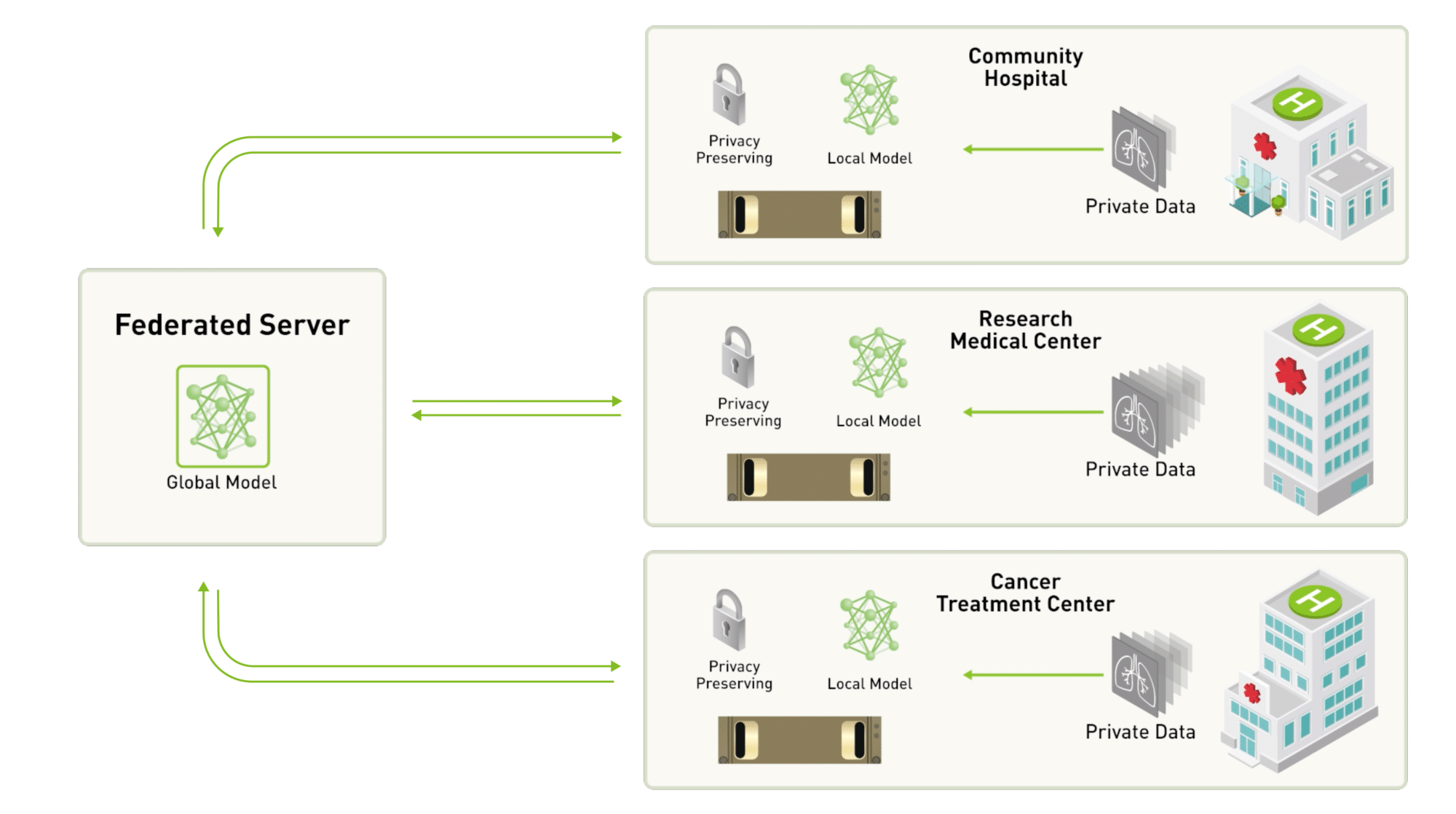
Federated learning by McMahan et al. (2017) is a form of distributed computing that involves training models on personal devices rather than centralizing the data on a single server (Figure 6.7). Initially, a base global model is trained on a central server to be distributed to all devices. Using this base model, the devices individually compute the gradients and send them back to the central hub. Intuitively, this transfers model parameters instead of the data itself. Federated learning enhances privacy by keeping sensitive data on local devices and only sharing model updates with a central server. This method is particularly useful when dealing with sensitive data or when a large-scale infrastructure is impractical.
However, federated learning faces challenges such as ensuring data accuracy, managing non-IID (independent and identically distributed) data, dealing with unbalanced data production, and overcoming communication overhead and device heterogeneity. Privacy and security concerns, such as gradient inversion attacks, also pose significant challenges.
Machine learning frameworks simplify the implementation of federated learning by providing necessary tools and libraries. For example, TensorFlow Federated (TFF) offers an open-source framework to support federated learning. TFF allows developers to simulate and implement federated learning algorithms, offering a federated core for low-level operations and high-level APIs for common federated tasks. It seamlessly integrates with TensorFlow, enabling the use of TensorFlow models and optimizers in a federated setting. TFF supports secure aggregation techniques to improve privacy and allows for customization of federated learning algorithms. By leveraging these tools, developers can efficiently distribute training, fine-tune pre-trained models, and handle federated learning’s inherent complexities.
Other open source programs such as Flower have also been developed to simplify implementing federated learning with various machine learning frameworks.
6.6 Framework Specialization
Thus far, we have talked about ML frameworks generally. However, typically, frameworks are optimized based on the target environment’s computational capabilities and application requirements, ranging from the cloud to the edge to tiny devices. Choosing the right framework is crucial based on the target environment for deployment. This section provides an overview of the major types of AI frameworks tailored for cloud, edge, and TinyML environments to help understand the similarities and differences between these ecosystems.
6.6.1 Cloud
Cloud-based AI frameworks assume access to ample computational power, memory, and storage resources in the cloud. They generally support both training and inference. Cloud-based AI frameworks are suited for applications where data can be sent to the cloud for processing, such as cloud-based AI services, large-scale data analytics, and web applications. Popular cloud AI frameworks include the ones we mentioned earlier, such as TensorFlow, PyTorch, MXNet, Keras, etc. These frameworks utilize GPUs, TPUs, distributed training, and AutoML to deliver scalable AI. Concepts like model serving, MLOps, and AIOps relate to the operationalization of AI in the cloud. Cloud AI powers services like Google Cloud AI and enables transfer learning using pre-trained models.
6.6.2 Edge
Edge AI frameworks are tailored to deploy AI models on IoT devices, smartphones, and edge servers. Edge AI frameworks are optimized for devices with moderate computational resources, balancing power and performance. Edge AI frameworks are ideal for applications requiring real-time or near-real-time processing, including robotics, autonomous vehicles, and smart devices. Key edge AI frameworks include TensorFlow Lite, PyTorch Mobile, CoreML, and others. They employ optimizations like model compression, quantization, and efficient neural network architectures. Hardware support includes CPUs, GPUs, NPUs, and accelerators like the Edge TPU. Edge AI enables use cases like mobile vision, speech recognition, and real-time anomaly detection.
6.6.3 Embedded
TinyML frameworks are specialized for deploying AI models on extremely resource-constrained devices, specifically microcontrollers and sensors within the IoT ecosystem. TinyML frameworks are designed for devices with limited resources, emphasizing minimal memory and power consumption. TinyML frameworks are specialized for use cases on resource-constrained IoT devices for predictive maintenance, gesture recognition, and environmental monitoring applications. Major TinyML frameworks include TensorFlow Lite Micro, uTensor, and ARM NN. They optimize complex models to fit within kilobytes of memory through techniques like quantization-aware training and reduced precision. TinyML allows intelligent sensing across battery-powered devices, enabling collaborative learning via federated learning. The choice of framework involves balancing model performance and computational constraints of the target platform, whether cloud, edge, or TinyML. Table 6.3 compares the major AI frameworks across cloud, edge, and TinyML environments:
| Framework Type | Examples | Key Technologies | Use Cases |
|---|---|---|---|
| Cloud AI | TensorFlow, PyTorch, MXNet, Keras | GPUs, TPUs, distributed training, AutoML, MLOps | Cloud services, web apps, big data analytics |
| Edge AI | TensorFlow Lite, PyTorch Mobile, Core ML | Model optimization, compression, quantization, efficient NN architectures | Mobile apps, autonomous systems, real-time processing |
| TinyML | TensorFlow Lite Micro, uTensor, ARM NN | Quantization-aware training, reduced precision, neural architecture search | IoT sensors, wearables, predictive maintenance, gesture recognition |
Key differences:
Cloud AI leverages massive computational power for complex models using GPUs/TPUs and distributed training
Edge AI optimizes models to run locally on resource-constrained edge devices.
TinyML fits models into extremely low memory and computes environments like microcontrollers
6.7 Embedded AI Frameworks
6.7.1 Resource Constraints
Embedded systems face severe resource constraints that pose unique challenges when deploying machine learning models compared to traditional computing platforms. For example, microcontroller units (MCUs) commonly used in IoT devices often have:
RAM ranges from tens of kilobytes to a few megabytes. The popular ESP8266 MCU has around 80KB RAM available to developers. This contrasts with 8GB or more on typical laptops and desktops today.
Flash storage ranges from hundreds of kilobytes to a few megabytes. The Arduino Uno microcontroller provides just 32KB of code storage. Standard computers today have disk storage in the order of terabytes.
Processing power from just a few MHz to approximately 200MHz. The ESP8266 operates at 80MHz. This is several orders of magnitude slower than multi-GHz multi-core CPUs in servers and high-end laptops.
These tight constraints often make training machine learning models directly on microcontrollers infeasible. The limited RAM precludes handling large datasets for training. Energy usage for training would also quickly deplete battery-powered devices. Instead, models are trained on resource-rich systems and deployed on microcontrollers for optimized inference. But even inference poses challenges:
Model Size: AI models are too large to fit on embedded and IoT devices. This necessitates model compression techniques, such as quantization, pruning, and knowledge distillation. Additionally, as we will see, many of the frameworks used by developers for AI development have large amounts of overhead and built-in libraries that embedded systems can’t support.
Complexity of Tasks: With only tens of KBs to a few MBs of RAM, IoT devices and embedded systems are constrained in the complexity of tasks they can handle. Tasks that require large datasets or sophisticated algorithms—for example, LLMs—that would run smoothly on traditional computing platforms might be infeasible on embedded systems without compression or other optimization techniques due to memory limitations.
Data Storage and Processing: Embedded systems often process data in real time and might only store small amounts locally. Conversely, traditional computing systems can hold and process large datasets in memory, enabling faster data operations analysis and real-time updates.
Security and Privacy: Limited memory also restricts the complexity of security algorithms and protocols, data encryption, reverse engineering protections, and more that can be implemented on the device. This could make some IoT devices more vulnerable to attacks.
Consequently, specialized software optimizations and ML frameworks tailored for microcontrollers must work within these tight resource bounds. Clever optimization techniques like quantization, pruning, and knowledge distillation compress models to fit within limited memory (see Optimizations section). Learnings from neural architecture search help guide model designs.
Hardware improvements like dedicated ML accelerators on microcontrollers also help alleviate constraints. For instance, Qualcomm’s Hexagon DSP accelerates TensorFlow Lite models on Snapdragon mobile chips. Google’s Edge TPU packs ML performance into a tiny ASIC for edge devices. ARM Ethos-U55 offers efficient inference on Cortex-M class microcontrollers. These customized ML chips unlock advanced capabilities for resource-constrained applications.
Due to limited processing power, it’s almost always infeasible to train AI models on IoT or embedded systems. Instead, models are trained on powerful traditional computers (often with GPUs) and then deployed on the embedded device for inference. TinyML specifically deals with this, ensuring models are lightweight enough for real-time inference on these constrained devices.
6.7.2 Frameworks & Libraries
Embedded AI frameworks are software tools and libraries designed to enable AI and ML capabilities on embedded systems. These frameworks are essential for bringing AI to IoT devices, robotics, and other edge computing platforms, and they are designed to work where computational resources, memory, and power consumption are limited.
6.7.3 Challenges
While embedded systems present an enormous opportunity for deploying machine learning to enable intelligent capabilities at the edge, these resource-constrained environments pose significant challenges. Unlike typical cloud or desktop environments rich with computational resources, embedded devices introduce severe constraints around memory, processing power, energy efficiency, and specialized hardware. As a result, existing machine learning techniques and frameworks designed for server clusters with abundant resources do not directly translate to embedded systems. This section uncovers some of the challenges and opportunities for embedded systems and ML frameworks.
Fragmented Ecosystem
The lack of a unified ML framework led to a highly fragmented ecosystem. Engineers at companies like STMicroelectronics, NXP Semiconductors, and Renesas had to develop custom solutions tailored to their specific microcontroller and DSP architectures. These ad-hoc frameworks required extensive manual optimization for each low-level hardware platform. This made porting models extremely difficult, requiring redevelopment for new Arm, RISC-V, or proprietary architectures.
Disparate Hardware Needs
Without a shared framework, there was no standard way to assess hardware’s capabilities. Vendors like Intel, Qualcomm, and NVIDIA created integrated solutions, blending models and improving software and hardware. This made it hard to discern the sources of performance gains - whether new chip designs like Intel’s low-power x86 cores or software optimizations were responsible. A standard framework was needed so vendors could evaluate their hardware’s capabilities fairly and reproducibly.
Lack of Portability
With standardized tools, adapting models trained in common frameworks like TensorFlow or PyTorch to run efficiently on microcontrollers was easier. It required time-consuming manual translation of models to run on specialized DSPs from companies like CEVA or low-power Arm M-series cores. No turnkey tools were enabling portable deployment across different architectures.
Incomplete Infrastructure
The infrastructure to support key model development workflows needed to be improved. More support is needed for compression techniques to fit large models within constrained memory budgets. Tools for quantization to lower precision for faster inference were missing. Standardized APIs for integration into applications were incomplete. Essential functionality like on-device debugging, metrics, and performance profiling was absent. These gaps increased the cost and difficulty of embedded ML development.
No Standard Benchmark
Without unified benchmarks, there was no standard way to assess and compare the capabilities of different hardware platforms from vendors like NVIDIA, Arm, and Ambiq Micro. Existing evaluations relied on proprietary benchmarks tailored to showcase the strengths of particular chips. This made it impossible to measure hardware improvements objectively in a fair, neutral manner. The Benchmarking AI chapter discusses this topic in more detail.
Minimal Real-World Testing
Much of the benchmarks relied on synthetic data. Rigorously testing models on real-world embedded applications was difficult without standardized datasets and benchmarks, raising questions about how performance claims would translate to real-world usage. More extensive testing was needed to validate chips in actual use cases.
The lack of shared frameworks and infrastructure slowed TinyML adoption, hampering the integration of ML into embedded products. Recent standardized frameworks have begun addressing these issues through improved portability, performance profiling, and benchmarking support. However, ongoing innovation is still needed to enable seamless, cost-effective deployment of AI to edge devices.
Summary
The absence of standardized frameworks, benchmarks, and infrastructure for embedded ML has traditionally hampered adoption. However, recent progress has been made in developing shared frameworks like TensorFlow Lite Micro and benchmark suites like MLPerf Tiny that aim to accelerate the proliferation of TinyML solutions. However, overcoming the fragmentation and difficulty of embedded deployment remains an ongoing process.
6.8 Examples
Machine learning deployment on microcontrollers and other embedded devices often requires specially optimized software libraries and frameworks to work within tight memory, compute, and power constraints. Several options exist for performing inference on such resource-limited hardware, each with its approach to optimizing model execution. This section will explore the key characteristics and design principles behind TFLite Micro, TinyEngine, and CMSIS-NN, providing insight into how each framework tackles the complex problem of high-accuracy yet efficient neural network execution on microcontrollers. It will also showcase different approaches for implementing efficient TinyML frameworks.
Table 6.4 summarizes the key differences and similarities between these three specialized machine-learning inference frameworks for embedded systems and microcontrollers.
| Framework | TensorFlow Lite Micro | TinyEngine | CMSIS-NN |
|---|---|---|---|
| Approach | Interpreter-based | Static compilation | Optimized neural network kernels |
| Hardware Focus | General embedded devices | Microcontrollers | ARM Cortex-M processors |
| Arithmetic Support | Floating point | Floating point, fixed point | Floating point, fixed point |
| Model Support | General neural network models | Models co-designed with TinyNAS | Common neural network layer types |
| Code Footprint | Larger due to inclusion of interpreter and ops | Small, includes only ops needed for model | Lightweight by design |
| Latency | Higher due to interpretation overhead | Very low due to compiled model | Low latency focus |
| Memory Management | Dynamically managed by interpreter | Model-level optimization | Tools for efficient allocation |
| Optimization Approach | Some code generation features | Specialized kernels, operator fusion | Architecture-specific assembly optimizations |
| Key Benefits | Flexibility, portability, ease of updating models | Maximizes performance, optimized memory usage | Hardware acceleration, standardized API, portability |
We will understand each of these in greater detail in the following sections.
6.8.1 Interpreter
TensorFlow Lite Micro (TFLM) is a machine learning inference framework designed for embedded devices with limited resources. It uses an interpreter to load and execute machine learning models, which provides flexibility and ease of updating models in the field (David et al. 2021).
Traditional interpreters often have significant branching overhead, which can reduce performance. However, machine learning model interpretation benefits from the efficiency of long-running kernels, where each kernel runtime is relatively large and helps mitigate interpreter overhead.
An alternative to an interpreter-based inference engine is to generate native code from a model during export. This can improve performance, but it sacrifices portability and flexibility, as the generated code needs recompilation for each target platform and must be replaced entirely to modify a model.
TFLM balances the simplicity of code compilation and the flexibility of an interpreter-based approach by incorporating certain code-generation features. For example, the library can be constructed solely from source files, offering much of the compilation simplicity associated with code generation while retaining the benefits of an interpreter-based model execution framework.
An interpreter-based approach offers several benefits over code generation for machine learning inference on embedded devices:
Flexibility: Models can be updated in the field without recompiling the entire application.
Portability: The interpreter can be used to execute models on different target platforms without porting the code.
Memory efficiency: The interpreter can share code across multiple models, reducing memory usage.
Ease of development: Interpreters are easier to develop and maintain than code generators.
TensorFlow Lite Micro is a powerful and flexible framework for machine learning inference on embedded devices. Its interpreter-based approach offers several benefits over code generation, including flexibility, portability, memory efficiency, and ease of development.
6.8.2 Compiler-based
TinyEngine is an ML inference framework designed specifically for resource-constrained microcontrollers. It employs several optimizations to enable high-accuracy neural network execution within the tight constraints of memory, computing, and storage on microcontrollers (Lin et al. 2020).
While inference frameworks like TFLite Micro use interpreters to execute the neural network graph dynamically at runtime, this adds significant overhead regarding memory usage to store metadata, interpretation latency, and lack of optimizations. However, TFLite argues that the overhead is small. TinyEngine eliminates this overhead by employing a code generation approach. It analyzes the network graph during compilation and generates specialized code to execute just that model. This code is natively compiled into the application binary, avoiding runtime interpretation costs.
Conventional ML frameworks schedule memory per layer, trying to minimize usage for each layer separately. TinyEngine does model-level scheduling instead of analyzing memory usage across layers. It allocates a common buffer size based on the maximum memory needs of all layers. This buffer is then shared efficiently across layers to increase data reuse.
TinyEngine also specializes in the kernels for each layer through techniques like tiling, unrolling, and fusing operators. For example, it will generate unrolled compute kernels with the number of loops needed for a 3x3 or 5x5 convolution. These specialized kernels extract maximum performance from the microcontroller hardware. It uses optimized depthwise convolutions to minimize memory allocations by computing each channel’s output in place over the input channel data. This technique exploits the channel-separable nature of depthwise convolutions to reduce peak memory size.
Like TFLite Micro, the compiled TinyEngine binary only includes operations needed for a specific model rather than all possible operations. This results in a very small binary footprint, keeping code size low for memory-constrained devices.
One difference between TFLite Micro and TinyEngine is that the latter is co-designed with “TinyNAS,” an architecture search method for microcontroller models similar to differential NAS for microcontrollers. TinyEngine’s efficiency allows for exploring larger and more accurate models through NAS. It also provides feedback to TinyNAS on which models can fit within the hardware constraints.
Through various custom techniques, such as static compilation, model-based scheduling, specialized kernels, and co-design with NAS, TinyEngine enables high-accuracy deep learning inference within microcontrollers’ tight resource constraints.
6.8.3 Library
CMSIS-NN, standing for Cortex Microcontroller Software Interface Standard for Neural Networks, is a software library devised by ARM. It offers a standardized interface for deploying neural network inference on microcontrollers and embedded systems, focusing on optimization for ARM Cortex-M processors (Lai, Suda, and Chandra 2018).
Neural Network Kernels: CMSIS-NN has highly efficient kernels that handle fundamental neural network operations such as convolution, pooling, fully connected layers, and activation functions. It caters to a broad range of neural network models by supporting floating and fixed-point arithmetic. The latter is especially beneficial for resource-constrained devices as it curtails memory and computational requirements (Quantization).
Hardware Acceleration: CMSIS-NN harnesses the power of Single Instruction, Multiple Data (SIMD) instructions available on many Cortex-M processors. This allows for parallel processing of multiple data elements within a single instruction, thereby boosting computational efficiency. Certain Cortex-M processors feature Digital Signal Processing (DSP) extensions that CMSIS-NN can exploit for accelerated neural network execution. The library also incorporates assembly-level optimizations tailored to specific microcontroller architectures to improve performance further.
Standardized API: CMSIS-NN offers a consistent and abstracted API that protects developers from the complexities of low-level hardware details. This makes the integration of neural network models into applications simpler. It may also encompass tools or utilities for converting popular neural network model formats into a format that is compatible with CMSIS-NN.
Memory Management: CMSIS-NN provides functions for efficient memory allocation and management, which is vital in embedded systems where memory resources are scarce. It ensures optimal memory usage during inference and, in some instances, allows in-place operations to decrease memory overhead.
Portability: CMSIS-NN is designed for portability across various Cortex-M processors. This enables developers to write code that can operate on different microcontrollers without significant modifications.
Low Latency: CMSIS-NN minimizes inference latency, making it an ideal choice for real-time applications where swift decision-making is paramount.
Energy Efficiency: The library is designed with a focus on energy efficiency, making it suitable for battery-powered and energy-constrained devices.
6.9 Choosing the Right Framework
Choosing the right machine learning framework for a given application requires carefully evaluating models, hardware, and software considerations. By analyzing these three aspects—models, hardware, and software—ML engineers can select the optimal framework and customize it as needed for efficient and performant on-device ML applications. The goal is to balance model complexity, hardware limitations, and software integration to design a tailored ML pipeline for embedded and edge devices.
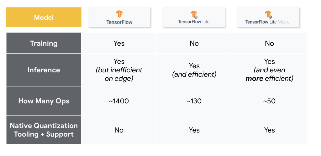
6.9.1 Model
TensorFlow supports significantly more operations (ops) than TensorFlow Lite and TensorFlow Lite Micro as it is typically used for research or cloud deployment, which require a large number of and more flexibility with operators (see Figure 6.8). TensorFlow Lite supports select ops for on-device training, whereas TensorFlow Micro does not. TensorFlow Lite also supports dynamic shapes and quantization-aware training, but TensorFlow Micro does not. In contrast, TensorFlow Lite and TensorFlow Micro offer native quantization tooling and support, where quantization refers to transforming an ML program into an approximated representation with available lower precision operations.
6.9.2 Software
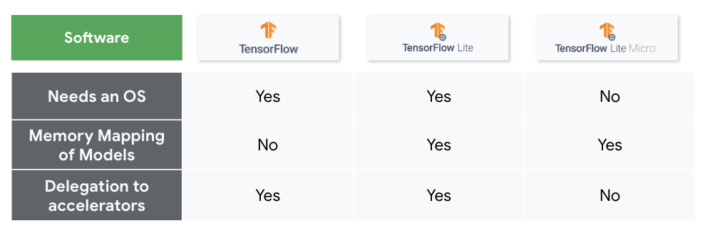
TensorFlow Lite Micro does not have OS support, while TensorFlow and TensorFlow Lite do, to reduce memory overhead, make startup times faster, and consume less energy (see Figure 6.9). TensorFlow Lite Micro can be used in conjunction with real-time operating systems (RTOS) like FreeRTOS, Zephyr, and Mbed OS. TensorFlow Lite and TensorFlow Lite Micro support model memory mapping, allowing models to be directly accessed from flash storage rather than loaded into RAM, whereas TensorFlow does not. TensorFlow and TensorFlow Lite support accelerator delegation to schedule code to different accelerators, whereas TensorFlow Lite Micro does not, as embedded systems tend to have a limited array of specialized accelerators.
6.9.3 Hardware
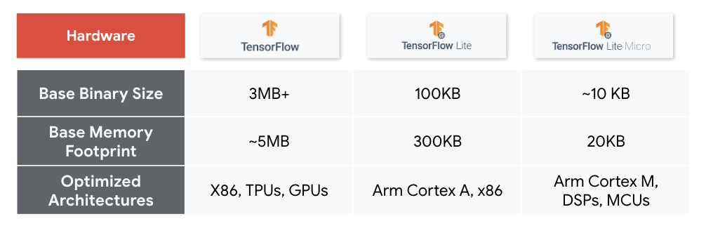
TensorFlow Lite and TensorFlow Lite Micro have significantly smaller base binary sizes and memory footprints than TensorFlow (see Figure 6.10). For example, a typical TensorFlow Lite Micro binary is less than 200KB, whereas TensorFlow is much larger. This is due to the resource-constrained environments of embedded systems. TensorFlow supports x86, TPUs, and GPUs like NVIDIA, AMD, and Intel. TensorFlow Lite supports Arm Cortex-A and x86 processors commonly used on mobile phones and tablets. The latter is stripped of all the unnecessary training logic for on-device deployment. TensorFlow Lite Micro provides support for microcontroller-focused Arm Cortex M cores like M0, M3, M4, and M7, as well as DSPs like Hexagon and SHARC and MCUs like STM32, NXP Kinetis, Microchip AVR.
6.9.4 Other Factors
Selecting the appropriate AI framework is essential to ensure that embedded systems can efficiently execute AI models. Several key factors beyond models, hardware, and software should be considered when evaluating AI frameworks for embedded systems. Other key factors to consider when choosing a machine learning framework are performance, scalability, ease of use, integration with data engineering tools, integration with model optimization tools, and community support. By understanding these factors, you can make informed decisions and maximize the potential of your machine-learning initiatives.
Performance
Performance is critical in embedded systems where computational resources are limited. Evaluate the framework’s ability to optimize model inference for embedded hardware. Model quantization and hardware acceleration support are crucial in achieving efficient inference.
Scalability
Scalability is essential when considering the potential growth of an embedded AI project. The framework should support the deployment of models on various embedded devices, from microcontrollers to more powerful processors. It should also seamlessly handle both small-scale and large-scale deployments.
Integration with Data Engineering Tools
Data engineering tools are essential for data preprocessing and pipeline management. An ideal AI framework for embedded systems should seamlessly integrate with these tools, allowing for efficient data ingestion, transformation, and model training.
Integration with Model Optimization Tools
Model optimization ensures that AI models are well-suited for embedded deployment. Evaluate whether the framework integrates with model optimization tools like TensorFlow Lite Converter or ONNX Runtime to facilitate model quantization and size reduction.
Ease of Use
The ease of use of an AI framework significantly impacts development efficiency. A framework with a user-friendly interface and clear documentation reduces developers’ learning curve. Consideration should be given to whether the framework supports high-level APIs, allowing developers to focus on model design rather than low-level implementation details. This factor is incredibly important for embedded systems, which have fewer features than typical developers might be accustomed to.
Community Support
Community support plays another essential factor. Frameworks with active and engaged communities often have well-maintained codebases, receive regular updates, and provide valuable forums for problem-solving. As a result, community support also plays into Ease of Use because it ensures that developers have access to a wealth of resources, including tutorials and example projects. Community support provides some assurance that the framework will continue to be supported for future updates. There are only a few frameworks that cater to TinyML needs. TensorFlow Lite Micro is the most popular and has the most community support.
6.10 Future Trends in ML Frameworks
6.10.1 Decomposition
Currently, the ML system stack consists of four abstractions as shown in Figure 6.11, namely (1) computational graphs, (2) tensor programs, (3) libraries and runtimes, and (4) hardware primitives.
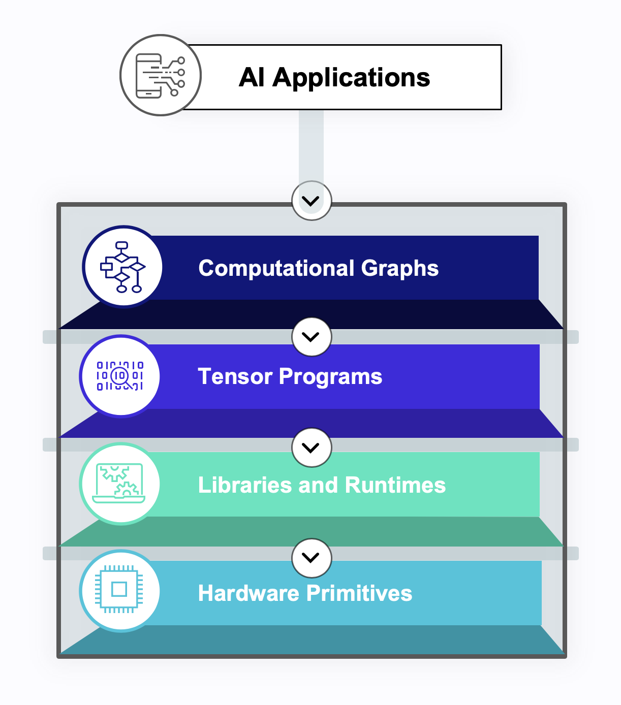
This has led to vertical (i.e., between abstraction levels) and horizontal (i.e., library-driven vs. compilation-driven approaches to tensor computation) boundaries, which hinder innovation for ML. Future work in ML frameworks can look toward breaking these boundaries. In December 2021, Apache TVM Unity was proposed, which aimed to facilitate interactions between the different abstraction levels (as well as the people behind them, such as ML scientists, ML engineers, and hardware engineers) and co-optimize decisions in all four abstraction levels.
6.10.2 High-Performance Compilers & Libraries
As ML frameworks further develop, high-performance compilers and libraries will continue to emerge. Some current examples include TensorFlow XLA and Nvidia’s CUTLASS, which accelerate linear algebra operations in computational graphs, and Nvidia’s TensorRT, which accelerates and optimizes inference.
6.10.3 ML for ML Frameworks
We can also use ML to improve ML frameworks in the future. Some current uses of ML for ML frameworks include:
Hyperparameter optimization using techniques such as Bayesian optimization, random search, and grid search
Neural Architecture Search (NAS) to automatically search for optimal network architectures
AutoML, which as described in Section 6.5, automates the ML pipeline.
6.11 Conclusion
In summary, selecting the optimal machine learning framework requires a thorough evaluation of various options against criteria such as usability, community support, performance, hardware compatibility, and model conversion capabilities. There is no one-size-fits-all solution, as the right framework depends on specific constraints and use cases.
We first introduced the necessity of machine learning frameworks like TensorFlow and PyTorch. These frameworks offer features such as tensors for handling multi-dimensional data, computational graphs for defining and optimizing model operations, and a suite of tools including loss functions, optimizers, and data loaders that streamline model development.
Advanced features further improve these frameworks’ usability, enabling tasks like fine-tuning large pre-trained models and facilitating federated learning. These capabilities are critical for developing sophisticated machine learning models efficiently.
Embedded AI frameworks, such as TensorFlow Lite Micro, provide specialized tools for deploying models on resource-constrained platforms. TensorFlow Lite Micro, for instance, offers comprehensive optimization tooling, including quantization mapping and kernel optimizations, to ensure high performance on microcontroller-based platforms like Arm Cortex-M and RISC-V processors. Frameworks specifically built for specialized hardware like CMSIS-NN on Cortex-M processors can further maximize performance but sacrifice portability. Integrated frameworks from processor vendors tailor the stack to their architectures, unlocking the full potential of their chips but locking you into their ecosystem.
Ultimately, choosing the right framework involves finding the best match between its capabilities and the requirements of the target platform. This requires balancing trade-offs between performance needs, hardware constraints, model complexity, and other factors. Thoroughly assessing the intended models and use cases and evaluating options against key metrics will guide developers in selecting the ideal framework for their machine learning applications.
6.12 Resources
Here is a curated list of resources to support students and instructors in their learning and teaching journeys. We are continuously working on expanding this collection and will add new exercises soon.
These slides are a valuable tool for instructors to deliver lectures and for students to review the material at their own pace. We encourage students and instructors to leverage these slides to improve their understanding and facilitate effective knowledge transfer.
- Coming soon.
To reinforce the concepts covered in this chapter, we have curated a set of exercises that challenge students to apply their knowledge and deepen their understanding.
In addition to exercises, we offer a series of hands-on labs allowing students to gain practical experience with embedded AI technologies. These labs provide step-by-step guidance, enabling students to develop their skills in a structured and supportive environment. We are excited to announce that new labs will be available soon, further enriching the learning experience.
- Coming soon.