17 Robust AI
Resources: Slides, Videos, Exercises, Labs

The development of robust machine learning systems has become increasingly crucial. As these systems are deployed in various critical applications, from autonomous vehicles to healthcare diagnostics, ensuring their resilience to faults and errors is paramount.
Robust AI, in the context of hardware faults, software faults, and errors, plays an important role in maintaining the reliability, safety, and performance of machine learning systems. By addressing the challenges posed by transient, permanent, and intermittent hardware faults (Ahmadilivani et al. 2024), as well as bugs, design flaws, and implementation errors in software (H. Zhang 2008), robust AI techniques enable machine learning systems to operate effectively even in adverse conditions.
This chapter explores the fundamental concepts, techniques, and tools for building fault-tolerant and error-resilient machine learning systems. It empowers researchers and practitioners to develop AI solutions that can withstand the complexities and uncertainties of real-world environments.
Understand the importance of robust and resilient AI systems in real-world applications.
Identify and characterize hardware faults, software faults, and their impact on ML systems.
Recognize and develop defensive strategies against threats posed by adversarial attacks, data poisoning, and distribution shifts.
Learn techniques for detecting, mitigating, and designing fault-tolerant ML systems.
Become familiar with tools and frameworks for studying and enhancing ML system resilience throughout the AI development lifecycle.
17.1 Introduction
Robust AI refers to a system’s ability to maintain its performance and reliability in the presence of errors. A robust machine learning system is designed to be fault-tolerant and error-resilient, capable of operating effectively even under adverse conditions.
As ML systems become increasingly integrated into various aspects of our lives, from cloud-based services to edge devices and embedded systems, the impact of hardware and software faults on their performance and reliability becomes more significant. In the future, as ML systems become more complex and are deployed in even more critical applications, the need for robust and fault-tolerant designs will be paramount.
ML systems are expected to play crucial roles in autonomous vehicles, smart cities, healthcare, and industrial automation domains. In these domains, the consequences of hardware or software faults can be severe, potentially leading to loss of life, economic damage, or environmental harm.
Researchers and engineers must focus on developing advanced techniques for fault detection, isolation, and recovery to mitigate these risks and ensure the reliable operation of future ML systems.
This chapter will focus specifically on three main categories of faults and errors that can impact the robustness of ML systems: hardware faults, software faults, and human errors.
Hardware Faults: Transient, permanent, and intermittent faults can affect the hardware components of an ML system, corrupting computations and degrading performance.
Model Robustness: ML models can be vulnerable to adversarial attacks, data poisoning, and distribution shifts, which can induce targeted misclassifications, skew the model’s learned behavior, or compromise the system’s integrity and reliability.
Software Faults: Bugs, design flaws, and implementation errors in the software components, such as algorithms, libraries, and frameworks, can propagate errors and introduce vulnerabilities.
The specific challenges and approaches to achieving robustness may vary depending on the scale and constraints of the ML system. Large-scale cloud computing or data center systems may focus on fault tolerance and resilience through redundancy, distributed processing, and advanced error detection and correction techniques. In contrast, resource-constrained edge devices or embedded systems face unique challenges due to limited computational power, memory, and energy resources.
Regardless of the scale and constraints, the key characteristics of a robust ML system include fault tolerance, error resilience, and performance maintenance. By understanding and addressing the multifaceted challenges to robustness, we can develop trustworthy and reliable ML systems that can navigate the complexities of real-world environments.
This chapter is not just about exploring ML systems’ tools, frameworks, and techniques for detecting and mitigating faults, attacks, and distributional shifts. It’s about emphasizing the crucial role of each one of you in prioritizing resilience throughout the AI development lifecycle, from data collection and model training to deployment and monitoring. By proactively addressing the challenges to robustness, we can unlock the full potential of ML technologies while ensuring their safe, reliable, and responsible deployment in real-world applications.
As AI continues to shape our future, the potential of ML technologies is immense. But it’s only when we build resilient systems that can withstand the challenges of the real world that we can truly harness this potential. This is a defining factor in the success and societal impact of this transformative technology, and it’s within our reach.
17.2 Real-World Examples
Here are some real-world examples of cases where faults in hardware or software have caused major issues in ML systems across cloud, edge, and embedded environments:
17.2.1 Cloud
In February 2017, Amazon Web Services (AWS) experienced a significant outage due to human error during maintenance. An engineer inadvertently entered an incorrect command, causing many servers to be taken offline. This outage disrupted many AWS services, including Amazon’s AI-powered assistant, Alexa. As a result, Alexa-powered devices, such as Amazon Echo and third-party products using Alexa Voice Service, could not respond to user requests for several hours. This incident highlights the potential impact of human errors on cloud-based ML systems and the need for robust maintenance procedures and failsafe mechanisms.
In another example (Vangal et al. 2021), Facebook encountered a silent data corruption (SDC) issue within its distributed querying infrastructure, as shown in Figure 17.1. Facebook’s infrastructure includes a querying system that fetches and executes SQL and SQL-like queries across multiple datasets using frameworks like Presto, Hive, and Spark. One of the applications that utilized this querying infrastructure was a compression application to reduce the footprint of data stores. In this compression application, files were compressed when not being read and decompressed when a read request was made. Before decompression, the file size was checked to ensure it was greater than zero, indicating a valid compressed file with contents.
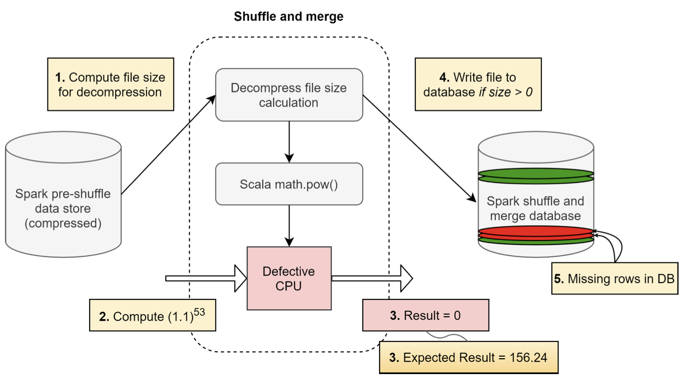
However, in one instance, when the file size was being computed for a valid non-zero-sized file, the decompression algorithm invoked a power function from the Scala library. Unexpectedly, the Scala function returned a zero size value for the file despite having a known non-zero decompressed size. As a result, the decompression was not performed, and the file was not written to the output database. This issue manifested sporadically, with some occurrences of the same file size computation returning the correct non-zero value.
The impact of this silent data corruption was significant, leading to missing files and incorrect data in the output database. The application relying on the decompressed files failed due to the data inconsistencies. In the case study presented in the paper, Facebook’s infrastructure, which consists of hundreds of thousands of servers handling billions of requests per day from their massive user base, encountered a silent data corruption issue. The affected system processed user queries, image uploads, and media content, which required fast, reliable, and secure execution.
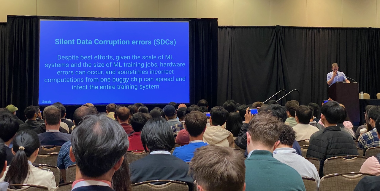
This case study illustrates how silent data corruption can propagate through multiple layers of an application stack, leading to data loss and application failures in a large-scale distributed system. The intermittent nature of the issue and the lack of explicit error messages made it particularly challenging to diagnose and resolve. But this is not restricted to just Meta, even other companies such as Google that operate AI hypercomputers face this challenge. Figure 17.2 Jeff Dean, Chief Scientist at Google DeepMind and Google Research, discusses SDCs and their impact on ML systems.
17.2.2 Edge
Regarding examples of faults and errors in edge ML systems, one area that has gathered significant attention is the domain of self-driving cars. Self-driving vehicles rely heavily on machine learning algorithms for perception, decision-making, and control, making them particularly susceptible to the impact of hardware and software faults. In recent years, several high-profile incidents involving autonomous vehicles have highlighted the challenges and risks associated with deploying these systems in real-world environments.
In May 2016, a fatal accident occurred when a Tesla Model S operating on Autopilot crashed into a white semi-trailer truck crossing the highway. The Autopilot system, which relied on computer vision and machine learning algorithms, failed to recognize the white trailer against a bright sky background. The driver, who was reportedly watching a movie when the crash, did not intervene in time, and the vehicle collided with the trailer at full speed. This incident raised concerns about the limitations of AI-based perception systems and the need for robust failsafe mechanisms in autonomous vehicles. It also highlighted the importance of driver awareness and the need for clear guidelines on using semi-autonomous driving features, as shown in Figure 17.3.

In March 2018, an Uber self-driving test vehicle struck and killed a pedestrian crossing the street in Tempe, Arizona. The incident was caused by a software flaw in the vehicle’s object recognition system, which failed to identify the pedestrians appropriately to avoid them as obstacles. The safety driver, who was supposed to monitor the vehicle’s operation and intervene if necessary, was found distracted during the crash. This incident led to widespread scrutiny of Uber’s self-driving program and raised questions about the readiness of autonomous vehicle technology for public roads. It also emphasized the need for rigorous testing, validation, and safety measures in developing and deploying AI-based self-driving systems.
In 2021, Tesla faced increased scrutiny following several accidents involving vehicles operating on Autopilot mode. Some of these accidents were attributed to issues with the Autopilot system’s ability to detect and respond to certain road situations, such as stationary emergency vehicles or obstacles in the road. For example, in April 2021, a Tesla Model S crashed into a tree in Texas, killing two passengers. Initial reports suggested that no one was in the driver’s seat at the time of the crash, raising questions about the use and potential misuse of Autopilot features. These incidents highlight the ongoing challenges in developing robust and reliable autonomous driving systems and the need for clear regulations and consumer education regarding the capabilities and limitations of these technologies.
17.2.3 Embedded
Embedded systems, which often operate in resource-constrained environments and safety-critical applications, have long faced challenges related to hardware and software faults. As AI and machine learning technologies are increasingly integrated into these systems, the potential for faults and errors takes on new dimensions, with the added complexity of AI algorithms and the critical nature of the applications in which they are deployed.
Let’s consider a few examples, starting with outer space exploration. NASA’s Mars Polar Lander mission in 1999 suffered a catastrophic failure due to a software error in the touchdown detection system (Figure 17.4). The spacecraft’s onboard software mistakenly interpreted the noise from the deployment of its landing legs as a sign that it had touched down on the Martian surface. As a result, the spacecraft prematurely shut down its engines, causing it to crash into the surface. This incident highlights the critical importance of robust software design and extensive testing in embedded systems, especially those operating in remote and unforgiving environments. As AI capabilities are integrated into future space missions, ensuring these systems’ reliability and fault tolerance will be paramount to mission success.

Back on earth, in 2015, a Boeing 787 Dreamliner experienced a complete electrical shutdown during a flight due to a software bug in its generator control units. This incident underscores the potential for software faults to have severe consequences in complex embedded systems like aircraft. As AI technologies are increasingly applied in aviation, such as in autonomous flight systems and predictive maintenance, ensuring the robustness and reliability of these systems will be critical to passenger safety.
“If the four main generator control units (associated with the engine-mounted generators) were powered up at the same time, after 248 days of continuous power, all four GCUs will go into failsafe mode at the same time, resulting in a loss of all AC electrical power regardless of flight phase.” – Federal Aviation Administration directive (2015)
As AI capabilities increasingly integrate into embedded systems, the potential for faults and errors becomes more complex and severe. Imagine a smart pacemaker that has a sudden glitch. A patient could die from that effect. Therefore, AI algorithms, such as those used for perception, decision-making, and control, introduce new sources of potential faults, such as data-related issues, model uncertainties, and unexpected behaviors in edge cases. Moreover, the opaque nature of some AI models can make it challenging to identify and diagnose faults when they occur.
17.3 Hardware Faults
Hardware faults are a significant challenge in computing systems, including traditional and ML systems. These faults occur when physical components, such as processors, memory modules, storage devices, or interconnects, malfunction or behave abnormally. Hardware faults can cause incorrect computations, data corruption, system crashes, or complete system failure, compromising the integrity and trustworthiness of the computations performed by the system (Jha et al. 2019). A complete system failure refers to a situation where the entire computing system becomes unresponsive or inoperable due to a critical hardware malfunction. This type of failure is the most severe, as it renders the system unusable and may lead to data loss or corruption, requiring manual intervention to repair or replace the faulty components.
Understanding the taxonomy of hardware faults is essential for anyone working with computing systems, especially in the context of ML systems. ML systems rely on complex hardware architectures and large-scale computations to train and deploy models that learn from data and make intelligent predictions or decisions. However, hardware faults can introduce errors and inconsistencies in the MLOps pipeline, affecting the trained models’ accuracy, robustness, and reliability (G. Li et al. 2017).
Knowing the different types of hardware faults, their mechanisms, and their potential impact on system behavior is crucial for developing effective strategies to detect, mitigate, and recover them. This knowledge is necessary for designing fault-tolerant computing systems, implementing robust ML algorithms, and ensuring the overall dependability of ML-based applications.
The following sections will explore the three main categories of hardware faults: transient, permanent, and intermittent. We will discuss their definitions, characteristics, causes, mechanisms, and examples of how they manifest in computing systems. We will also cover detection and mitigation techniques specific to each fault type.
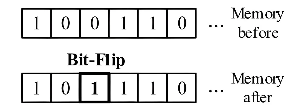
Transient Faults: Transient faults are temporary and non-recurring. They are often caused by external factors such as cosmic rays, electromagnetic interference, or power fluctuations. A common example of a transient fault is a bit flip, where a single bit in a memory location or register changes its value unexpectedly. Transient faults can lead to incorrect computations or data corruption, but they do not cause permanent damage to the hardware.
Permanent Faults: Permanent faults, also called hard errors, are irreversible and persist over time. They are typically caused by physical defects or wear-out of hardware components. Examples of permanent faults include stuck-at faults, where a bit or signal is permanently set to a specific value (e.g., always 0 or always 1), and device failures, such as a malfunctioning processor or a damaged memory module. Permanent faults can result in complete system failure or significant performance degradation.
Intermittent Faults: Intermittent faults are recurring faults that appear and disappear intermittently. Unstable hardware conditions, such as loose connections, aging components, or manufacturing defects, often cause them. Intermittent faults can be challenging to diagnose and reproduce because they may occur sporadically and under specific conditions. Examples include intermittent short circuits or contact resistance issues. Intermittent faults can lead to unpredictable system behavior and intermittent errors.
By the end of this discussion, readers will have a solid understanding of fault taxonomy and its relevance to traditional computing and ML systems. This foundation will help them make informed decisions when designing, implementing, and deploying fault-tolerant solutions, improving the reliability and trustworthiness of their computing systems and ML applications.
17.3.1 Transient Faults
Transient faults in hardware can manifest in various forms, each with its own unique characteristics and causes. These faults are temporary in nature and do not result in permanent damage to the hardware components.
Definition and Characteristics
Some of the common types of transient faults include Single Event Upsets (SEUs) caused by ionizing radiation, voltage fluctuations (Reddi and Gupta 2013) due to power supply noise or electromagnetic interference, Electromagnetic Interference (EMI) induced by external electromagnetic fields, Electrostatic Discharge (ESD) resulting from sudden static electricity flow, crosstalk caused by unintended signal coupling, ground bounce triggered by simultaneous switching of multiple outputs, timing violations due to signal timing constraint breaches, and soft errors in combinational logic affecting the output of logic circuits (Mukherjee, Emer, and Reinhardt 2005). Understanding these different types of transient faults is crucial for designing robust and resilient hardware systems that can mitigate their impact and ensure reliable operation.
All of these transient faults are characterized by their short duration and non-permanent nature. They do not persist or leave any lasting impact on the hardware. However, they can still lead to incorrect computations, data corruption, or system misbehavior if not properly handled.
Causes of Transient Faults
Transient faults can be attributed to various external factors. One common cause is cosmic rays, high-energy particles originating from outer space. When these particles strike sensitive areas of the hardware, such as memory cells or transistors, they can induce charge disturbances that alter the stored or transmitted data. This is illustrated in Figure 17.5. Another cause of transient faults is electromagnetic interference (EMI) from nearby devices or power fluctuations. EMI can couple with the circuits and cause voltage spikes or glitches that temporarily disrupt the normal operation of the hardware.
Mechanisms of Transient Faults
Transient faults can manifest through different mechanisms depending on the affected hardware component. In memory devices like DRAM or SRAM, transient faults often lead to bit flips, where a single bit changes its value from 0 to 1 or vice versa. This can corrupt the stored data or instructions. In logic circuits, transient faults can cause glitches or voltage spikes propagating through the combinational logic, resulting in incorrect outputs or control signals. Transient faults can also affect communication channels, causing bit errors or packet losses during data transmission.
Impact on ML Systems
A common example of a transient fault is a bit flip in the main memory. If an important data structure or critical instruction is stored in the affected memory location, it can lead to incorrect computations or program misbehavior. If a transient fault occurs in the memory storing the model weights or gradients. For instance, a bit flip in the memory storing a loop counter can cause the loop to execute indefinitely or terminate prematurely. Transient faults in control registers or flag bits can alter the flow of program execution, leading to unexpected jumps or incorrect branch decisions. In communication systems, transient faults can corrupt transmitted data packets, resulting in retransmissions or data loss.
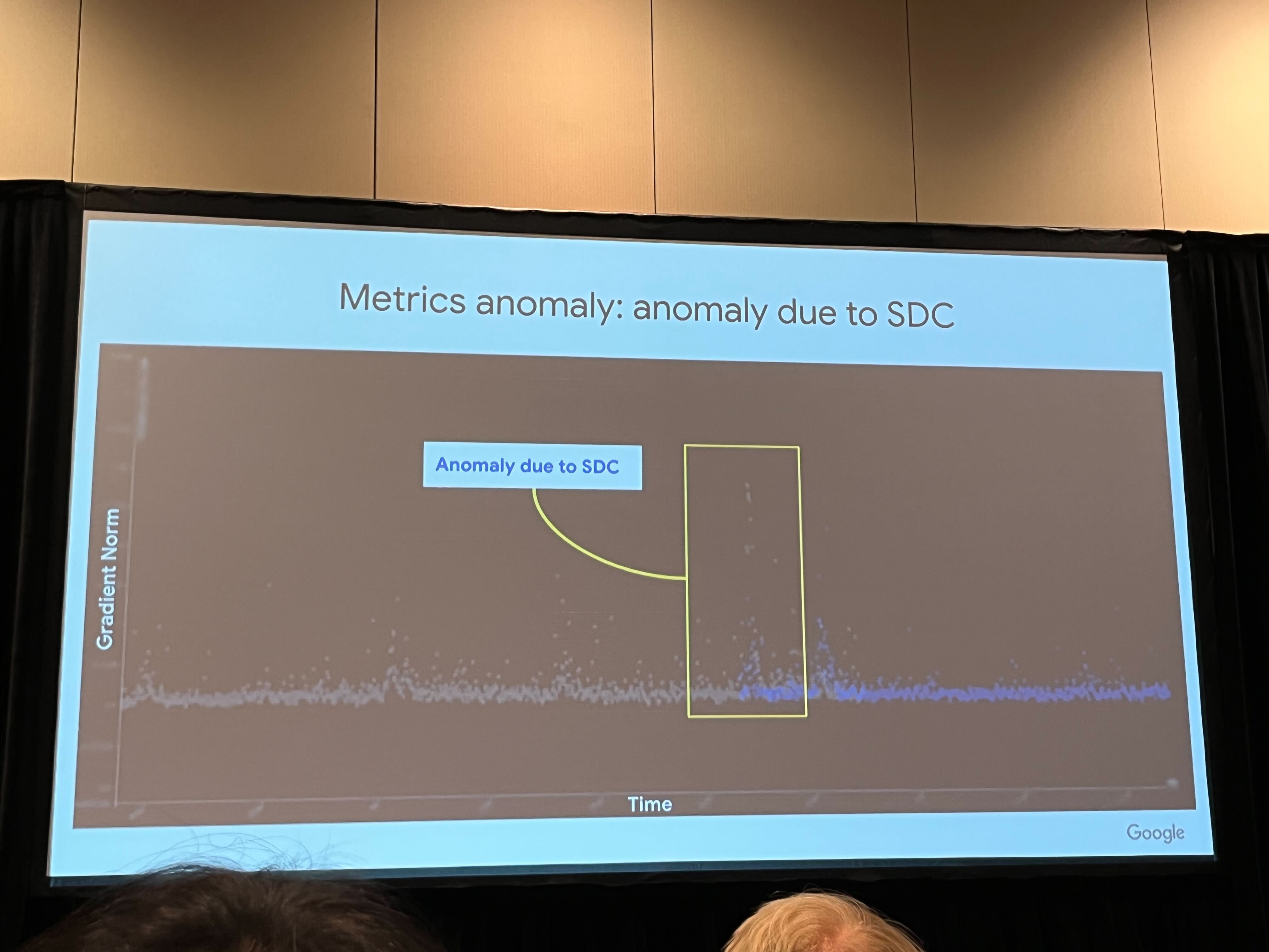
In ML systems, transient faults can have significant implications during the training phase (He et al. 2023). ML training involves iterative computations and updates to model parameters based on large datasets. If a transient fault occurs in the memory storing the model weights or gradients, it can lead to incorrect updates and compromise the convergence and accuracy of the training process. Figure 17.6 show a real-world example from Google’s production fleet where an SDC anomaly caused a significant difference in the gradient norm.
For example, a bit flip in the weight matrix of a neural network can cause the model to learn incorrect patterns or associations, leading to degraded performance (Wan et al. 2021). Transient faults in the data pipeline, such as corruption of training samples or labels, can also introduce noise and affect the quality of the learned model.
During the inference phase, transient faults can impact the reliability and trustworthiness of ML predictions. If a transient fault occurs in the memory storing the trained model parameters or in the computation of the inference results, it can lead to incorrect or inconsistent predictions. For instance, a bit flip in the activation values of a neural network can alter the final classification or regression output (Mahmoud et al. 2020).
In safety-critical applications, such as autonomous vehicles or medical diagnosis, transient faults during inference can have severe consequences, leading to incorrect decisions or actions (G. Li et al. 2017; Jha et al. 2019). Ensuring the resilience of ML systems against transient faults is crucial to maintaining the integrity and reliability of the predictions.
At the other extreme, in resource-constrained environments like TinyML, Binarized Neural Networks [BNNs] (Courbariaux et al. 2016) have emerged as a promising solution. BNNs represent network weights in single-bit precision, offering computational efficiency and faster inference times. However, this binary representation renders BNNs fragile to bit-flip errors on the network weights. For instance, prior work (Aygun, Gunes, and De Vleeschouwer 2021) has shown that a two-hidden layer BNN architecture for a simple task such as MNIST classification suffers performance degradation from 98% test accuracy to 70% when random bit-flipping soft errors are inserted through model weights with a 10% probability.
Addressing such issues requires considering flip-aware training techniques or leveraging emerging computing paradigms (e.g., stochastic computing) to improve fault tolerance and robustness, which we will discuss in Section 17.3.4. Future research directions aim to develop hybrid architectures, novel activation functions, and loss functions tailored to bridge the accuracy gap compared to full-precision models while maintaining their computational efficiency.
17.3.2 Permanent Faults
Permanent faults are hardware defects that persist and cause irreversible damage to the affected components. These faults are characterized by their persistent nature and require repair or replacement of the faulty hardware to restore normal system functionality.
Definition and Characteristics
Permanent faults are hardware defects that cause persistent and irreversible malfunctions in the affected components. The faulty component remains non-operational until a permanent fault is repaired or replaced. These faults are characterized by their consistent and reproducible nature, meaning that the faulty behavior is observed every time the affected component is used. Permanent faults can impact various hardware components, such as processors, memory modules, storage devices, or interconnects, leading to system crashes, data corruption, or complete system failure.
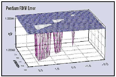
One notable example of a permanent fault is the Intel FDIV bug, which was discovered in 1994. The FDIV bug was a flaw in certain Intel Pentium processors’ floating-point division (FDIV) units. The bug caused incorrect results for specific division operations, leading to inaccurate calculations.
The FDIV bug occurred due to an error in the lookup table used by the division unit. In rare cases, the processor would fetch an incorrect value from the lookup table, resulting in a slightly less precise result than expected. For instance, Figure 17.7 shows a fraction 4195835/3145727 plotted on a Pentium processor with the FDIV permanent fault. The triangular regions are where erroneous calculations occurred. Ideally, all correct values would round to 1.3338, but the erroneous results show 1.3337, indicating a mistake in the 5th digit.
Although the error was small, it could compound over many division operations, leading to significant inaccuracies in mathematical calculations. The impact of the FDIV bug was significant, especially for applications that relied heavily on precise floating-point division, such as scientific simulations, financial calculations, and computer-aided design. The bug led to incorrect results, which could have severe consequences in fields like finance or engineering.
The Intel FDIV bug is a cautionary tale for the potential impact of permanent faults on ML systems. In the context of ML, permanent faults in hardware components can lead to incorrect computations, affecting the accuracy and reliability of the models. For example, if an ML system relies on a processor with a faulty floating-point unit, similar to the Intel FDIV bug, it could introduce errors in the calculations performed during training or inference.
These errors can propagate through the model, leading to inaccurate predictions or skewed learning. In applications where ML is used for critical tasks, such as autonomous driving, medical diagnosis, or financial forecasting, the consequences of incorrect computations due to permanent faults can be severe.
It is crucial for ML practitioners to be aware of the potential impact of permanent faults and to incorporate fault-tolerant techniques, such as hardware redundancy, error detection and correction mechanisms, and robust algorithm design, to mitigate the risks associated with these faults. Additionally, thorough testing and validation of ML hardware components can help identify and address permanent faults before they impact the system’s performance and reliability.
Causes of Permanent Faults
Permanent faults can arise from several causes, including manufacturing defects and wear-out mechanisms. Manufacturing defects are inherent flaws introduced during the fabrication process of hardware components. These defects include improper etching, incorrect doping, or contamination, leading to non-functional or partially functional components.
On the other hand, wear-out mechanisms occur over time as the hardware components are subjected to prolonged use and stress. Factors such as electromigration, oxide breakdown, or thermal stress can cause gradual degradation of the components, eventually leading to permanent failures.
Mechanisms of Permanent Faults
Permanent faults can manifest through various mechanisms, depending on the nature and location of the fault. Stuck-at faults (Seong et al. 2010) are common permanent faults where a signal or memory cell remains fixed at a particular value (either 0 or 1) regardless of the inputs, as illustrated in Figure 17.8.
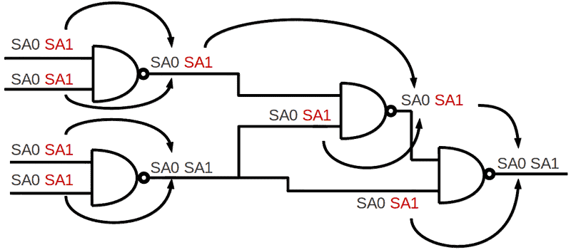
Stuck-at faults can occur in logic gates, memory cells, or interconnects, causing incorrect computations or data corruption. Another mechanism is device failures, where a component, such as a transistor or a memory cell, completely ceases to function. This can be due to manufacturing defects or severe wear-out. Bridging faults occur when two or more signal lines are unintentionally connected, causing short circuits or incorrect logic behavior.
In addition to stuck-at faults, there are several other types of permanent faults that can affect digital circuits that can impact an ML system. Delay faults can cause the propagation delay of a signal to exceed the specified limit, leading to timing violations. Interconnect faults, such as open faults (broken wires), resistive faults (increased resistance), or capacitive faults (increased capacitance), can cause signal integrity issues or timing violations. Memory cells can also suffer from various faults, including transition faults (inability to change state), coupling faults (interference between adjacent cells), and neighborhood pattern sensitive faults (faults that depend on the values of neighboring cells). Other permanent faults can occur in the power supply network or the clock distribution network, affecting the functionality and timing of the circuit.
Impact on ML Systems
Permanent faults can severely affect the behavior and reliability of computing systems. For example, a stuck-at-fault in a processor’s arithmetic logic unit (ALU) can cause incorrect computations, leading to erroneous results or system crashes. A permanent fault in a memory module, such as a stuck-at fault in a specific memory cell, can corrupt the stored data, causing data loss or program misbehavior. In storage devices, permanent faults like bad sectors or device failures can result in data inaccessibility or complete loss of stored information. Permanent interconnect faults can disrupt communication channels, causing data corruption or system hangs.
Permanent faults can significantly affect ML systems during the training and inference phases. During training, permanent faults in processing units or memory can lead to incorrect computations, resulting in corrupted or suboptimal models (He et al. 2023). Furthermore, faults in storage devices can corrupt the training data or the stored model parameters, leading to data loss or model inconsistencies (He et al. 2023).
During inference, permanent faults can impact the reliability and correctness of ML predictions. Faults in the processing units can produce incorrect results or cause system failures, while faults in memory storing the model parameters can lead to corrupted or outdated models being used for inference (J. J. Zhang et al. 2018).
To mitigate the impact of permanent faults in ML systems, fault-tolerant techniques must be employed at both the hardware and software levels. Hardware redundancy, such as duplicating critical components or using error-correcting codes (Kim, Sullivan, and Erez 2015), can help detect and recover from permanent faults. Software techniques, such as checkpoint and restart mechanisms (Egwutuoha et al. 2013), can enable the system to recover from permanent faults by returning to a previously saved state. Regular monitoring, testing, and maintenance of ML systems can help identify and replace faulty components before they cause significant disruptions.
Designing ML systems with fault tolerance in mind is crucial to ensure their reliability and robustness in the presence of permanent faults. This may involve incorporating redundancy, error detection and correction mechanisms, and fail-safe strategies into the system architecture. By proactively addressing the challenges posed by permanent faults, ML systems can maintain their integrity, accuracy, and trustworthiness, even in the face of hardware failures.
17.3.3 Intermittent Faults
Intermittent faults are hardware faults that occur sporadically and unpredictably in a system. An example is illustrated in Figure 17.9, where cracks in the material can introduce increased resistance in circuitry. These faults are particularly challenging to detect and diagnose because they appear and disappear intermittently, making it difficult to reproduce and isolate the root cause. Intermittent faults can lead to system instability, data corruption, and performance degradation.

Definition and Characteristics
Intermittent faults are characterized by their sporadic and non-deterministic nature. They occur irregularly and may appear and disappear spontaneously, with varying durations and frequencies. These faults do not consistently manifest every time the affected component is used, making them harder to detect than permanent faults. Intermittent faults can affect various hardware components, including processors, memory modules, storage devices, or interconnects. They can cause transient errors, data corruption, or unexpected system behavior.
Intermittent faults can significantly impact the behavior and reliability of computing systems (Rashid, Pattabiraman, and Gopalakrishnan 2015). For example, an intermittent fault in a processor’s control logic can cause irregular program flow, leading to incorrect computations or system hangs. Intermittent faults in memory modules can corrupt data values, resulting in erroneous program execution or data inconsistencies. In storage devices, intermittent faults can cause read/write errors or data loss. Intermittent faults in communication channels can lead to data corruption, packet loss, or intermittent connectivity issues. These faults can cause system crashes, data integrity problems, or performance degradation, depending on the severity and frequency of the intermittent failures.
Causes of Intermittent Faults
Intermittent faults can arise from several causes, both internal and external, to the hardware components (Constantinescu 2008). One common cause is aging and wear-out of the components. As electronic devices age, they become more susceptible to intermittent failures due to degradation mechanisms such as electromigration, oxide breakdown, or solder joint fatigue.
Manufacturing defects or process variations can also introduce intermittent faults, where marginal or borderline components may exhibit sporadic failures under specific conditions, as shown in Figure 17.10.
Environmental factors, such as temperature fluctuations, humidity, or vibrations, can trigger intermittent faults by altering the electrical characteristics of the components. Loose or degraded connections, such as those in connectors or printed circuit boards, can cause intermittent faults.

Mechanisms of Intermittent Faults
Intermittent faults can manifest through various mechanisms, depending on the underlying cause and the affected component. One mechanism is the intermittent open or short circuit, where a signal path or connection becomes temporarily disrupted or shorted, causing erratic behavior. Another mechanism is the intermittent delay fault (J. Zhang et al. 2018), where the timing of signals or propagation delays becomes inconsistent, leading to synchronization issues or incorrect computations. Intermittent faults can manifest as transient bit flips or soft errors in memory cells or registers, causing data corruption or incorrect program execution.
Impact on ML Systems
In the context of ML systems, intermittent faults can introduce significant challenges and impact the system’s reliability and performance. During the training phase, intermittent faults in processing units or memory can lead to inconsistencies in computations, resulting in incorrect or noisy gradients and weight updates. This can affect the convergence and accuracy of the training process, leading to suboptimal or unstable models. Intermittent data storage or retrieval faults can corrupt the training data, introducing noise or errors that degrade the quality of the learned models (He et al. 2023).
During the inference phase, intermittent faults can impact the reliability and consistency of ML predictions. Faults in the processing units or memory can cause incorrect computations or data corruption, leading to erroneous or inconsistent predictions. Intermittent faults in the data pipeline can introduce noise or errors in the input data, affecting the accuracy and robustness of the predictions. In safety-critical applications, such as autonomous vehicles or medical diagnosis systems, intermittent faults can have severe consequences, leading to incorrect decisions or actions that compromise safety and reliability.
Mitigating the impact of intermittent faults in ML systems requires a multifaceted approach (Rashid, Pattabiraman, and Gopalakrishnan 2012). At the hardware level, techniques such as robust design practices, component selection, and environmental control can help reduce the occurrence of intermittent faults. Redundancy and error correction mechanisms can be employed to detect and recover from intermittent failures. At the software level, runtime monitoring, anomaly detection, and fault-tolerant techniques can be incorporated into the ML pipeline. This may include techniques such as data validation, outlier detection, model ensembling, or runtime model adaptation to handle intermittent faults gracefully.
Designing ML systems resilient to intermittent faults is crucial to ensuring their reliability and robustness. This involves incorporating fault-tolerant techniques, runtime monitoring, and adaptive mechanisms into the system architecture. By proactively addressing the challenges of intermittent faults, ML systems can maintain their accuracy, consistency, and trustworthiness, even in sporadic hardware failures. Regular testing, monitoring, and maintenance of ML systems can help identify and mitigate intermittent faults before they cause significant disruptions or performance degradation.
17.3.4 Detection and Mitigation
This section explores various fault detection techniques, including hardware-level and software-level approaches, and discusses effective mitigation strategies to enhance the resilience of ML systems. Additionally, we will look into resilient ML system design considerations, present case studies and examples, and highlight future research directions in fault-tolerant ML systems.
Fault Detection Techniques
Fault detection techniques are important for identifying and localizing hardware faults in ML systems. These techniques can be broadly categorized into hardware-level and software-level approaches, each offering unique capabilities and advantages.
Hardware-level fault detection
Hardware-level fault detection techniques are implemented at the physical level of the system and aim to identify faults in the underlying hardware components. There are several hardware techniques, but broadly, we can bucket these different mechanisms into the following categories.
Built-in self-test (BIST) mechanisms: BIST is a powerful technique for detecting faults in hardware components (Bushnell and Agrawal 2002). It involves incorporating additional hardware circuitry into the system for self-testing and fault detection. BIST can be applied to various components, such as processors, memory modules, or application-specific integrated circuits (ASICs). For example, BIST can be implemented in a processor using scan chains, which are dedicated paths that allow access to internal registers and logic for testing purposes.
During the BIST process, predefined test patterns are applied to the processor’s internal circuitry, and the responses are compared against expected values. Any discrepancies indicate the presence of faults. Intel’s Xeon processors, for instance, include BIST mechanisms to test the CPU cores, cache memory, and other critical components during system startup.
Error detection codes: Error detection codes are widely used to detect data storage and transmission errors (Hamming 1950). These codes add redundant bits to the original data, allowing the detection of bit errors. Example: Parity checks are a simple form of error detection code shown in Figure 17.11. In a single-bit parity scheme, an extra bit is appended to each data word, making the number of 1s in the word even (even parity) or odd (odd parity).

When reading the data, the parity is checked, and if it doesn’t match the expected value, an error is detected. More advanced error detection codes, such as cyclic redundancy checks (CRC), calculate a checksum based on the data and append it to the message. The checksum is recalculated at the receiving end and compared with the transmitted checksum to detect errors. Error-correcting code (ECC) memory modules, commonly used in servers and critical systems, employ advanced error detection and correction codes to detect and correct single-bit or multi-bit errors in memory.
Hardware redundancy and voting mechanisms: Hardware redundancy involves duplicating critical components and comparing their outputs to detect and mask faults (Sheaffer, Luebke, and Skadron 2007). Voting mechanisms, such as triple modular redundancy (TMR), employ multiple instances of a component and compare their outputs to identify and mask faulty behavior (Arifeen, Hassan, and Lee 2020).
In a TMR system, three identical instances of a hardware component, such as a processor or a sensor, perform the same computation in parallel. The outputs of these instances are fed into a voting circuit, which compares the results and selects the majority value as the final output. If one of the instances produces an incorrect result due to a fault, the voting mechanism masks the error and maintains the correct output. TMR is commonly used in aerospace and aviation systems, where high reliability is critical. For instance, the Boeing 777 aircraft employs TMR in its primary flight computer system to ensure the availability and correctness of flight control functions (Yeh 1996).
Tesla’s self-driving computers employ a redundant hardware architecture to ensure the safety and reliability of critical functions, such as perception, decision-making, and vehicle control, as shown in Figure 17.12. One key component of this architecture is using dual modular redundancy (DMR) in the car’s onboard computer systems.

In Tesla’s DMR implementation, two identical hardware units, often called “redundant computers” or “redundant control units,” perform the same computations in parallel (Bannon et al. 2019). Each unit independently processes sensor data, executes perception and decision-making algorithms, and generates control commands for the vehicle’s actuators (e.g., steering, acceleration, and braking).
The outputs of these two redundant units are continuously compared to detect any discrepancies or faults. If the outputs match, the system assumes that both units function correctly, and the control commands are sent to the vehicle’s actuators. However, if there is a mismatch between the outputs, the system identifies a potential fault in one of the units and takes appropriate action to ensure safe operation.
The system may employ additional mechanisms to determine which unit is faulty in a mismatch. This can involve using diagnostic algorithms, comparing the outputs with data from other sensors or subsystems, or analyzing the consistency of the outputs over time. Once the faulty unit is identified, the system can isolate it and continue operating using the output from the non-faulty unit.
DMR in Tesla’s self-driving computer provides an extra safety and fault tolerance layer. By having two independent units performing the same computations, the system can detect and mitigate faults that may occur in one of the units. This redundancy helps prevent single points of failure and ensures that critical functions remain operational despite hardware faults.
Furthermore, Tesla also incorporates additional redundancy mechanisms beyond DMR. For example, they use redundant power supplies, steering and braking systems, and diverse sensor suites (e.g., cameras, radar, and ultrasonic sensors) to provide multiple layers of fault tolerance. These redundancies collectively contribute to the overall safety and reliability of the self-driving system.
It’s important to note that while DMR provides fault detection and some level of fault tolerance, TMR may provide a different level of fault masking. In DMR, if both units experience simultaneous faults or the fault affects the comparison mechanism, the system may be unable to identify the fault. Therefore, Tesla’s SDCs rely on a combination of DMR and other redundancy mechanisms to achieve a high level of fault tolerance.
The use of DMR in Tesla’s self-driving computer highlights the importance of hardware redundancy in safety-critical applications. By employing redundant computing units and comparing their outputs, the system can detect and mitigate faults, enhancing the overall safety and reliability of the self-driving functionality.
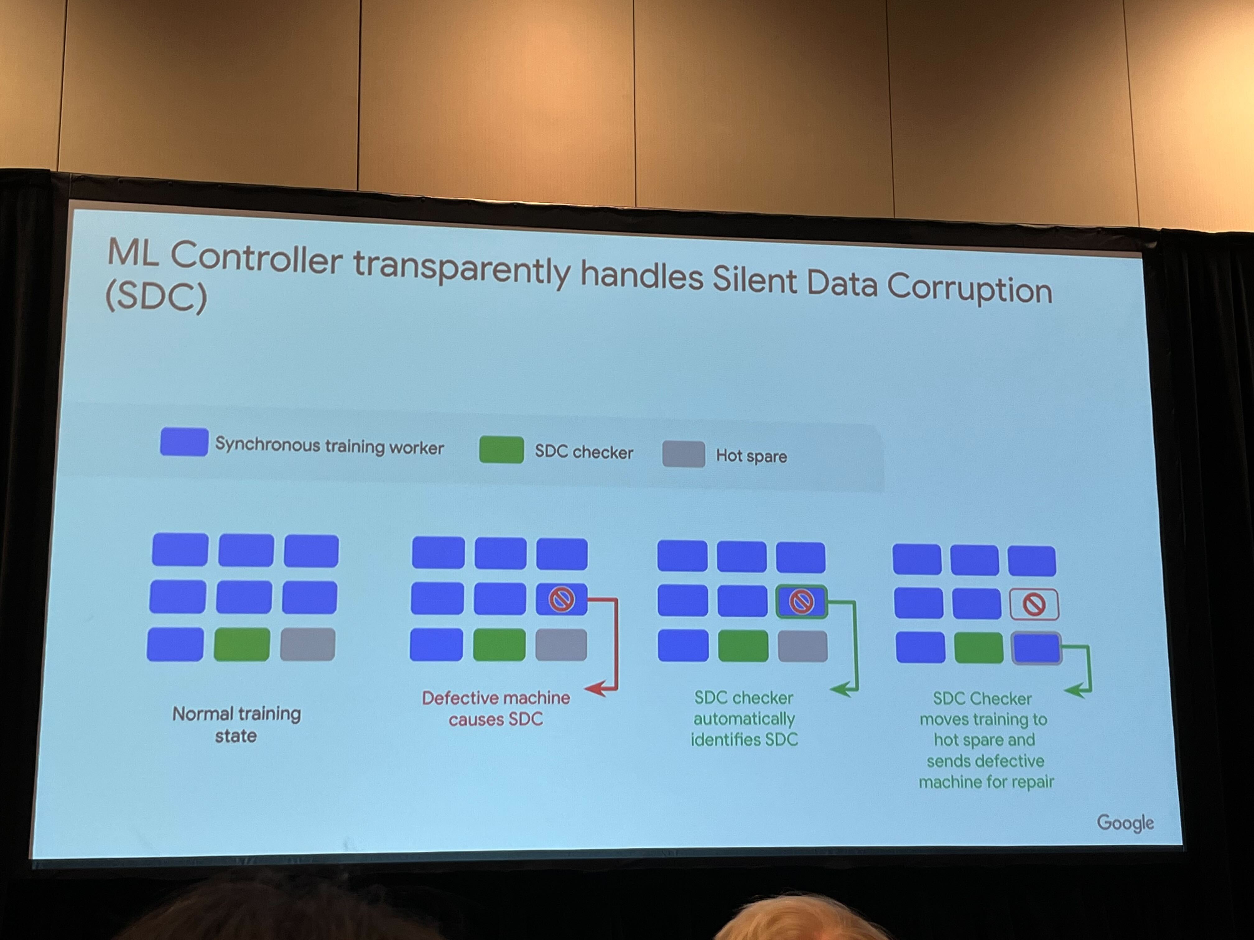
Google employs redundant hot spares to deal with SDC issues within its data centers, thereby enhancing the reliability of critical functions. As illustrated in Figure 17.13, during the normal training phase, multiple synchronous training workers function flawlessly. However, if a worker becomes defective and causes SDC, an SDC checker automatically identifies the issues. Upon detecting the SDC, the SDC checker moves the training to a hot spare and sends the defective machine for repair. This redundancy safeguards the continuity and reliability of ML training, effectively minimizing downtime and preserving data integrity.
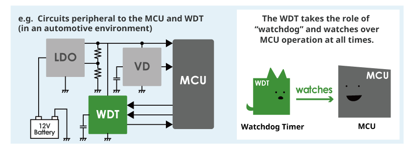
Watchdog timers: Watchdog timers are hardware components that monitor the execution of critical tasks or processes (Pont and Ong 2002). They are commonly used to detect and recover from software or hardware faults that cause a system to become unresponsive or stuck in an infinite loop. In an embedded system, a watchdog timer can be configured to monitor the execution of the main control loop, as illustrated in Figure 17.14. The software periodically resets the watchdog timer to indicate that it functions correctly. Suppose the software fails to reset the timer within a specified time limit (timeout period). In that case, the watchdog timer assumes that the system has encountered a fault and triggers a predefined recovery action, such as resetting the system or switching to a backup component. Watchdog timers are widely used in automotive electronics, industrial control systems, and other safety-critical applications to ensure the timely detection and recovery from faults.
Software-level fault detection
Software-level fault detection techniques rely on software algorithms and monitoring mechanisms to identify system faults. These techniques can be implemented at various levels of the software stack, including the operating system, middleware, or application level.
Runtime monitoring and anomaly detection: Runtime monitoring involves continuously observing the behavior of the system and its components during execution (Francalanza et al. 2017). It helps detect anomalies, errors, or unexpected behavior that may indicate the presence of faults. For example, consider an ML-based image classification system deployed in a self-driving car. Runtime monitoring can be implemented to track the classification model’s performance and behavior (Mahmoud et al. 2021).
Anomaly detection algorithms can be applied to the model’s predictions or intermediate layer activations, such as statistical outlier detection or machine learning-based approaches (e.g., One-Class SVM or Autoencoders) (Chandola, Banerjee, and Kumar 2009). Figure 17.15 shows example of anomaly detection. Suppose the monitoring system detects a significant deviation from the expected patterns, such as a sudden drop in classification accuracy or out-of-distribution samples. In that case, it can raise an alert indicating a potential fault in the model or the input data pipeline. This early detection allows for timely intervention and fault mitigation strategies to be applied.
Consistency checks and data validation: Consistency checks and data validation techniques ensure data integrity and correctness at different processing stages in an ML system (Lindholm et al. 2019). These checks help detect data corruption, inconsistencies, or errors that may propagate and affect the system’s behavior. Example: In a distributed ML system where multiple nodes collaborate to train a model, consistency checks can be implemented to validate the integrity of the shared model parameters. Each node can compute a checksum or hash of the model parameters before and after the training iteration, as shown in Figure 17.15. Any inconsistencies or data corruption can be detected by comparing the checksums across nodes. Additionally, range checks can be applied to the input data and model outputs to ensure they fall within expected bounds. For instance, if an autonomous vehicle’s perception system detects an object with unrealistic dimensions or velocities, it can indicate a fault in the sensor data or the perception algorithms (Wan et al. 2023).
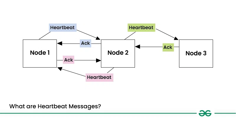
Heartbeat and timeout mechanisms: Heartbeat mechanisms and timeouts are commonly used to detect faults in distributed systems and ensure the liveness and responsiveness of components (Kawazoe Aguilera, Chen, and Toueg 1997). These are quite similar to the watchdog timers found in hardware. For example, in a distributed ML system, where multiple nodes collaborate to perform tasks such as data preprocessing, model training, or inference, heartbeat mechanisms can be implemented to monitor the health and availability of each node. Each node periodically sends a heartbeat message to a central coordinator or its peer nodes, indicating its status and availability. Suppose a node fails to send a heartbeat within a specified timeout period, as shown in Figure 17.16. In that case, it is considered faulty, and appropriate actions can be taken, such as redistributing the workload or initiating a failover mechanism. Timeouts can also be used to detect and handle hanging or unresponsive components. For example, if a data loading process exceeds a predefined timeout threshold, it may indicate a fault in the data pipeline, and the system can take corrective measures.
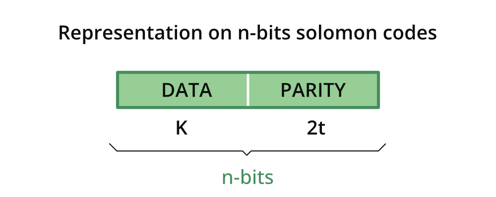
Software-implemented fault tolerance (SIFT) techniques: SIFT techniques introduce redundancy and fault detection mechanisms at the software level to improve the reliability and fault tolerance of the system (Reis et al. 2005). Example: N-version programming is a SIFT technique where multiple functionally equivalent software component versions are developed independently by different teams. This can be applied to critical components such as the model inference engine in an ML system. Multiple versions of the inference engine can be executed in parallel, and their outputs can be compared for consistency. It is considered the correct result if most versions produce the same output. If there is a discrepancy, it indicates a potential fault in one or more versions, and appropriate error-handling mechanisms can be triggered. Another example is using software-based error correction codes, such as Reed-Solomon codes (Plank 1997), to detect and correct errors in data storage or transmission, as shown in Figure 17.17. These codes add redundancy to the data, enabling detecting and correcting certain errors and enhancing the system’s fault tolerance.
In this Colab, play the role of an AI fault detective! You’ll build an autoencoder-based anomaly detector to pinpoint errors in heart health data. Learn how to identify malfunctions in ML systems, a vital skill for creating dependable AI. We’ll use Keras Tuner to fine-tune your autoencoder for top-notch fault detection. This experience directly links to the Robust AI chapter, demonstrating the importance of fault detection in real-world applications like healthcare and autonomous systems. Get ready to strengthen the reliability of your AI creations!
![]()
17.3.5 Summary
Table 17.1 provides an extensive comparative analysis of transient, permanent, and intermittent faults. It outlines the primary characteristics or dimensions that distinguish these fault types. Here, we summarize the relevant dimensions we examined and explore the nuances that differentiate transient, permanent, and intermittent faults in greater detail.
| Dimension | Transient Faults | Permanent Faults | Intermittent Faults |
|---|---|---|---|
| Duration | Short-lived, temporary | Persistent, remains until repair or replacement | Sporadic, appears and disappears intermittently |
| Persistence | Disappears after the fault condition passes | Consistently present until addressed | Recurs irregularly, not always present |
| Causes | External factors (e.g., electromagnetic interference cosmic rays) | Hardware defects, physical damage, wear-out | Unstable hardware conditions, loose connections, aging components |
| Manifestation | Bit flips, glitches, temporary data corruption | Stuck-at faults, broken components, complete device failures | Occasional bit flips, intermittent signal issues, sporadic malfunctions |
| Impact on ML Systems | Introduces temporary errors or noise in computations | Causes consistent errors or failures, affecting reliability | Leads to sporadic and unpredictable errors, challenging to diagnose and mitigate |
| Detection | Error detection codes, comparison with expected values | Built-in self-tests, error detection codes, consistency checks | Monitoring for anomalies, analyzing error patterns and correlations |
| Mitigation | Error correction codes, redundancy, checkpoint and restart | Hardware repair or replacement, component redundancy, failover mechanisms | Robust design, environmental control, runtime monitoring, fault-tolerant techniques |
17.4 ML Model Robustness
17.4.1 Adversarial Attacks
Definition and Characteristics
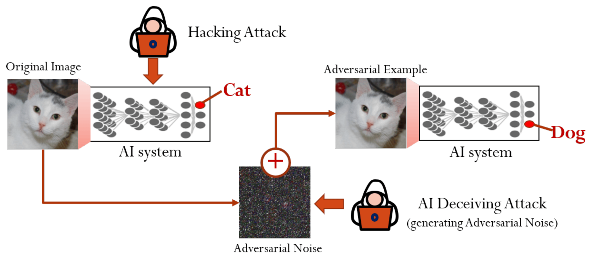
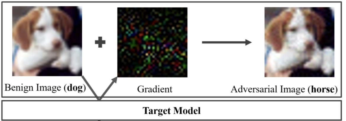
Adversarial attacks aim to trick models into making incorrect predictions by providing them with specially crafted, deceptive inputs (called adversarial examples) (Parrish et al. 2023). By adding slight perturbations to input data, adversaries can “hack” a model’s pattern recognition and deceive it. These are sophisticated techniques where slight, often imperceptible alterations to input data can trick an ML model into making a wrong prediction, as shown in Figure 17.18.
One can generate prompts that lead to unsafe images in text-to-image models like DALLE (Ramesh et al. 2021) or Stable Diffusion (Rombach et al. 2022). For example, by altering the pixel values of an image, attackers can deceive a facial recognition system into identifying a face as a different person.
Adversarial attacks exploit the way ML models learn and make decisions during inference. These models work on the principle of recognizing patterns in data. An adversary crafts special inputs with perturbations to mislead the model’s pattern recognition—essentially ‘hacking’ the model’s perceptions.
Adversarial attacks fall under different scenarios:
Whitebox Attacks: The attacker fully knows the target model’s internal workings, including the training data, parameters, and architecture (Ye and Hamidi 2021). This comprehensive access creates favorable conditions for attackers to exploit the model’s vulnerabilities. The attacker can use specific and subtle weaknesses to craft effective adversarial examples.
Blackbox Attacks: In contrast to white-box attacks, black-box attacks involve the attacker having little to no knowledge of the target model (Guo et al. 2019). To carry out the attack, the adversarial actor must carefully observe the model’s output behavior.
Greybox Attacks: These fall between blackbox and whitebox attacks. The attacker has only partial knowledge about the target model’s internal design (Xu et al. 2021). For example, the attacker could have knowledge about training data but not the architecture or parameters. In the real world, practical attacks typically fall under black-box or grey-box categories.
The landscape of machine learning models is complex and broad, especially given their relatively recent integration into commercial applications. This rapid adoption, while transformative, has brought to light numerous vulnerabilities within these models. Consequently, various adversarial attack methods have emerged, each strategically exploiting different aspects of different models. Below, we highlight a subset of these methods, showcasing the multifaceted nature of adversarial attacks on machine learning models:
Generative Adversarial Networks (GANs) are deep learning models that consist of two networks competing against each other: a generator and a discriminator (Goodfellow et al. 2020). The generator tries to synthesize realistic data while the discriminator evaluates whether they are real or fake. GANs can be used to craft adversarial examples. The generator network is trained to produce inputs that the target model misclassifies. These GAN-generated images can then attack a target classifier or detection model. The generator and the target model are engaged in a competitive process, with the generator continually improving its ability to create deceptive examples and the target model enhancing its resistance to such examples. GANs provide a powerful framework for crafting complex and diverse adversarial inputs, illustrating the adaptability of generative models in the adversarial landscape.
Transfer Learning Adversarial Attacks exploit the knowledge transferred from a pre-trained model to a target model, creating adversarial examples that can deceive both models. These attacks pose a growing concern, particularly when adversaries have knowledge of the feature extractor but lack access to the classification head (the part or layer responsible for making the final classifications). Referred to as “headless attacks,” these transferable adversarial strategies leverage the expressive capabilities of feature extractors to craft perturbations while being oblivious to the label space or training data. The existence of such attacks underscores the importance of developing robust defenses for transfer learning applications, especially since pre-trained models are commonly used (Abdelkader et al. 2020).
Mechanisms of Adversarial Attacks
Gradient-based Attacks
One prominent category of adversarial attacks is gradient-based attacks. These attacks leverage the gradients of the ML model’s loss function to craft adversarial examples. The Fast Gradient Sign Method (FGSM) is a well-known technique in this category. FGSM perturbs the input data by adding small noise in the gradient direction, aiming to maximize the model’s prediction error. FGSM can quickly generate adversarial examples, as shown in Figure 17.19, by taking a single step in the gradient direction.
Another variant, the Projected Gradient Descent (PGD) attack, extends FGSM by iteratively applying the gradient update step, allowing for more refined and powerful adversarial examples. The Jacobian-based Saliency Map Attack (JSMA) is another gradient-based approach that identifies the most influential input features and perturbs them to create adversarial examples.
Optimization-based Attacks
These attacks formulate the generation of adversarial examples as an optimization problem. The Carlini and Wagner (C&W) attack is a prominent example in this category. It finds the smallest perturbation that can cause misclassification while maintaining the perceptual similarity to the original input. The C&W attack employs an iterative optimization process to minimize the perturbation while maximizing the model’s prediction error.
Another optimization-based approach is the Elastic Net Attack to DNNs (EAD), which incorporates elastic net regularization to generate adversarial examples with sparse perturbations.
Transfer-based Attacks
Transfer-based attacks exploit the transferability property of adversarial examples. Transferability refers to the phenomenon where adversarial examples crafted for one ML model can often fool other models, even if they have different architectures or were trained on different datasets. This enables attackers to generate adversarial examples using a surrogate model and then transfer them to the target model without requiring direct access to its parameters or gradients. Transfer-based attacks highlight the generalization of adversarial vulnerabilities across different models and the potential for black-box attacks.
Physical-world Attacks
Physical-world attacks bring adversarial examples into the realm of real-world scenarios. These attacks involve creating physical objects or manipulations that can deceive ML models when captured by sensors or cameras. Adversarial patches, for example, are small, carefully designed patches that can be placed on objects to fool object detection or classification models. When attached to real-world objects, these patches can cause models to misclassify or fail to detect the objects accurately. Adversarial objects, such as 3D-printed sculptures or modified road signs, can also be crafted to deceive ML systems in physical environments.
Summary
Table 17.2 a concise overview of the different categories of adversarial attacks, including gradient-based attacks (FGSM, PGD, JSMA), optimization-based attacks (C&W, EAD), transfer-based attacks, and physical-world attacks (adversarial patches and objects). Each attack is briefly described, highlighting its key characteristics and mechanisms.
| Attack Category | Attack Name | Description |
|---|---|---|
| Gradient-based | Fast Gradient Sign Method (FGSM) Projected Gradient Descent (PGD) Jacobian-based Saliency Map Attack (JSMA) | Perturbs input data by adding small noise in the gradient direction to maximize prediction error. Extends FGSM by iteratively applying the gradient update step for more refined adversarial examples. Identifies influential input features and perturbs them to create adversarial examples. |
| Optimization-based | Carlini and Wagner (C&W) Attack Elastic Net Attack to DNNs (EAD) | Finds the smallest perturbation that causes misclassification while maintaining perceptual similarity. Incorporates elastic net regularization to generate adversarial examples with sparse perturbations. |
| Transfer-based | Transferability-based Attacks | Exploits the transferability of adversarial examples across different models, enabling black-box attacks. |
| Physical-world | Adversarial Patches Adversarial Objects | Small, carefully designed patches placed on objects to fool object detection or classification models. Physical objects (e.g., 3D-printed sculptures, modified road signs) crafted to deceive ML systems in real-world scenarios. |
The mechanisms of adversarial attacks reveal the intricate interplay between the ML model’s decision boundaries, the input data, and the attacker’s objectives. By carefully manipulating the input data, attackers can exploit the model’s sensitivities and blind spots, leading to incorrect predictions. The success of adversarial attacks highlights the need for a deeper understanding of ML models’ robustness and generalization properties.
Defending against adversarial attacks requires a multifaceted approach. Adversarial training is one common defense strategy in which models are trained on adversarial examples to improve robustness. Exposing the model to adversarial examples during training teaches it to classify them correctly and become more resilient to attacks. Defensive distillation, input preprocessing, and ensemble methods are other techniques that can help mitigate the impact of adversarial attacks.
As adversarial machine learning evolves, researchers explore new attack mechanisms and develop more sophisticated defenses. The arms race between attackers and defenders drives the need for constant innovation and vigilance in securing ML systems against adversarial threats. Understanding the mechanisms of adversarial attacks is crucial for developing robust and reliable ML models that can withstand the ever-evolving landscape of adversarial examples.
Impact on ML Systems
Adversarial attacks on machine learning systems have emerged as a significant concern in recent years, highlighting the potential vulnerabilities and risks associated with the widespread adoption of ML technologies. These attacks involve carefully crafted perturbations to input data that can deceive or mislead ML models, leading to incorrect predictions or misclassifications, as shown in Figure 17.20. The impact of adversarial attacks on ML systems is far-reaching and can have serious consequences in various domains.
One striking example of the impact of adversarial attacks was demonstrated by researchers in 2017. They experimented with small black and white stickers on stop signs (Eykholt et al. 2017). To the human eye, these stickers did not obscure the sign or prevent its interpretability. However, when images of the sticker-modified stop signs were fed into standard traffic sign classification ML models, a shocking result emerged. The models misclassified the stop signs as speed limit signs over 85% of the time.
This demonstration shed light on the alarming potential of simple adversarial stickers to trick ML systems into misreading critical road signs. The implications of such attacks in the real world are significant, particularly in the context of autonomous vehicles. If deployed on actual roads, these adversarial stickers could cause self-driving cars to misinterpret stop signs as speed limits, leading to dangerous situations, as shown in Figure 17.21. Researchers warned that this could result in rolling stops or unintended acceleration into intersections, endangering public safety.


The case study of the adversarial stickers on stop signs provides a concrete illustration of how adversarial examples exploit how ML models recognize patterns. By subtly manipulating the input data in ways that are invisible to humans, attackers can induce incorrect predictions and create serious risks, especially in safety-critical applications like autonomous vehicles. The attack’s simplicity highlights the vulnerability of ML models to even minor changes in the input, emphasizing the need for robust defenses against such threats.
The impact of adversarial attacks extends beyond the degradation of model performance. These attacks raise significant security and safety concerns, particularly in domains where ML models are relied upon for critical decision-making. In healthcare applications, adversarial attacks on medical imaging models could lead to misdiagnosis or incorrect treatment recommendations, jeopardizing patient well-being (M.-J. Tsai, Lin, and Lee 2023). In financial systems, adversarial attacks could enable fraud or manipulation of trading algorithms, resulting in substantial economic losses.
Moreover, adversarial vulnerabilities undermine the trustworthiness and interpretability of ML models. If carefully crafted perturbations can easily fool models, confidence in their predictions and decisions erodes. Adversarial examples expose the models’ reliance on superficial patterns and the inability to capture the true underlying concepts, challenging the reliability of ML systems (Fursov et al. 2021).
Defending against adversarial attacks often requires additional computational resources and can impact the overall system performance. Techniques like adversarial training, where models are trained on adversarial examples to improve robustness, can significantly increase training time and computational requirements (Bai et al. 2021). Runtime detection and mitigation mechanisms, such as input preprocessing (Addepalli et al. 2020) or prediction consistency checks, introduce latency and affect the real-time performance of ML systems.
The presence of adversarial vulnerabilities also complicates the deployment and maintenance of ML systems. System designers and operators must consider the potential for adversarial attacks and incorporate appropriate defenses and monitoring mechanisms. Regular updates and retraining of models become necessary to adapt to new adversarial techniques and maintain system security and performance over time.
The impact of adversarial attacks on ML systems is significant and multifaceted. These attacks expose ML models’ vulnerabilities, from degrading model performance and raising security and safety concerns to challenging model trustworthiness and interpretability. Developers and researchers must prioritize the development of robust defenses and countermeasures to mitigate the risks posed by adversarial attacks. By addressing these challenges, we can build more secure, reliable, and trustworthy ML systems that can withstand the ever-evolving landscape of adversarial threats.
Get ready to become an AI adversary! In this Colab, you’ll become a white-box hacker, learning to craft attacks that deceive image classification models. We’ll focus on the Fast Gradient Sign Method (FGSM), where you’ll weaponize a model’s gradients against it! You’ll deliberately distort images with tiny perturbations, observing how they increasingly fool the AI more intensely. This hands-on exercise highlights the importance of building secure AI – a critical skill as AI integrates into cars and healthcare. The Colab directly ties into the Robust AI chapter of your book, moving adversarial attacks from theory into your own hands-on experience.
![]()
Think you can outsmart an AI? In this Colab, learn how to trick image classification models with adversarial attacks. We’ll use methods like FGSM to change images and subtly fool the AI. Discover how to design deceptive image patches and witness the surprising vulnerability of these powerful models. This is crucial knowledge for building truly robust AI systems!
![]()
17.4.2 Data Poisoning
Definition and Characteristics
Data poisoning is an attack where the training data is tampered with, leading to a compromised model (Biggio, Nelson, and Laskov 2012), as shown in Figure 17.22. Attackers can modify existing training examples, insert new malicious data points, or influence the data collection process. The poisoned data is labeled in such a way as to skew the model’s learned behavior. This can be particularly damaging in applications where ML models make automated decisions based on learned patterns. Beyond training sets, poisoning tests, and validation data can allow adversaries to boost reported model performance artificially.

The process usually involves the following steps:
Injection: The attacker adds incorrect or misleading examples into the training set. These examples are often designed to look normal to cursory inspection but have been carefully crafted to disrupt the learning process.
Training: The ML model trains on this manipulated dataset and develops skewed understandings of the data patterns.
Deployment: Once the model is deployed, the corrupted training leads to flawed decision-making or predictable vulnerabilities the attacker can exploit.
The impact of data poisoning extends beyond classification errors or accuracy drops. In critical applications like healthcare, such alterations can lead to significant trust and safety issues (Marulli, Marrone, and Verde 2022). Later, we will discuss a few case studies of these issues.
There are six main categories of data poisoning (Oprea, Singhal, and Vassilev 2022):
Availability Attacks: These attacks aim to compromise the overall functionality of a model. They cause it to misclassify most testing samples, rendering the model unusable for practical applications. An example is label flipping, where labels of a specific, targeted class are replaced with labels from a different one.
Targeted Attacks: In contrast to availability attacks, targeted attacks aim to compromise a small number of the testing samples. So, the effect is localized to a limited number of classes, while the model maintains the same original level of accuracy for the majority of the classes. The targeted nature of the attack requires the attacker to possess knowledge of the model’s classes, making detecting these attacks more challenging.
Backdoor Attacks: In these attacks, an adversary targets specific patterns in the data. The attacker introduces a backdoor (a malicious, hidden trigger or pattern) into the training data, such as manipulating certain features in structured data or manipulating a pattern of pixels at a fixed position. This causes the model to associate the malicious pattern with specific labels. As a result, when the model encounters test samples that contain a malicious pattern, it makes false predictions.
Subpopulation Attacks: Attackers selectively choose to compromise a subset of the testing samples while maintaining accuracy on the rest of the samples. You can think of these attacks as a combination of availability and targeted attacks: performing availability attacks (performance degradation) within the scope of a targeted subset. Although subpopulation attacks may seem very similar to targeted attacks, the two have clear differences:
Scope: While targeted attacks target a selected set of samples, subpopulation attacks target a general subpopulation with similar feature representations. For example, in a targeted attack, an actor inserts manipulated images of a ‘speed bump’ warning sign (with carefully crafted perturbations or patterns), which causes an autonomous car to fail to recognize such a sign and slow down. On the other hand, manipulating all samples of people with a British accent so that a speech recognition model would misclassify a British person’s speech is an example of a subpopulation attack.
Knowledge: While targeted attacks require a high degree of familiarity with the data, subpopulation attacks require less intimate knowledge to be effective.
The characteristics of data poisoning include:
Subtle and hard-to-detect manipulations of training data: Data poisoning often involves subtle manipulations of the training data that are carefully crafted to be difficult to detect through casual inspection. Attackers employ sophisticated techniques to ensure that the poisoned samples blend seamlessly with the legitimate data, making them easier to identify with thorough analysis. These manipulations can target specific features or attributes of the data, such as altering numerical values, modifying categorical labels, or introducing carefully designed patterns. The goal is to influence the model’s learning process while evading detection, allowing the poisoned data to subtly corrupt the model’s behavior.
Can be performed by insiders or external attackers: Data poisoning attacks can be carried out by various actors, including malicious insiders with access to the training data and external attackers who find ways to influence the data collection or preprocessing pipeline. Insiders pose a significant threat because they often have privileged access and knowledge of the system, enabling them to introduce poisoned data without raising suspicions. On the other hand, external attackers may exploit vulnerabilities in data sourcing, crowdsourcing platforms, or data aggregation processes to inject poisoned samples into the training dataset. This highlights the importance of implementing strong access controls, data governance policies, and monitoring mechanisms to mitigate the risk of insider threats and external attacks.
Exploits vulnerabilities in data collection and preprocessing: Data poisoning attacks often exploit vulnerabilities in the machine learning pipeline’s data collection and preprocessing stages. Attackers carefully design poisoned samples to evade common data validation techniques, ensuring that the manipulated data still falls within acceptable ranges, follows expected distributions, or maintains consistency with other features. This allows the poisoned data to pass through data preprocessing steps without detection. Furthermore, poisoning attacks can take advantage of weaknesses in data preprocessing, such as inadequate data cleaning, insufficient outlier detection, or lack of integrity checks. Attackers may also exploit the lack of robust data provenance and lineage tracking mechanisms to introduce poisoned data without leaving a traceable trail. Addressing these vulnerabilities requires rigorous data validation, anomaly detection, and data provenance tracking techniques to ensure the integrity and trustworthiness of the training data.
Disrupts the learning process and skews model behavior: Data poisoning attacks are designed to disrupt the learning process of machine learning models and skew their behavior towards the attacker’s objectives. The poisoned data is typically manipulated with specific goals, such as skewing the model’s behavior towards certain classes, introducing backdoors, or degrading overall performance. These manipulations are not random but targeted to achieve the attacker’s desired outcomes. By introducing label inconsistencies, where the manipulated samples have labels that do not align with their true nature, poisoning attacks can confuse the model during training and lead to biased or incorrect predictions. The disruption caused by poisoned data can have far-reaching consequences, as the compromised model may make flawed decisions or exhibit unintended behavior when deployed in real-world applications.
Impacts model performance, fairness, and trustworthiness: Poisoned data in the training dataset can have severe implications for machine learning models’ performance, fairness, and trustworthiness. Poisoned data can degrade the accuracy and performance of the trained model, leading to increased misclassifications or errors in predictions. This can have significant consequences, especially in critical applications where the model’s outputs inform important decisions. Moreover, poisoning attacks can introduce biases and fairness issues, causing the model to make discriminatory or unfair decisions for certain subgroups or classes. This undermines machine learning systems’ ethical and social responsibilities and can perpetuate or amplify existing biases. Furthermore, poisoned data erodes the trustworthiness and reliability of the entire ML system. The model’s outputs become questionable and potentially harmful, leading to a loss of confidence in the system’s integrity. The impact of poisoned data can propagate throughout the entire ML pipeline, affecting downstream components and decisions that rely on the compromised model. Addressing these concerns requires robust data governance, regular model auditing, and ongoing monitoring to detect and mitigate the effects of data poisoning attacks.
Mechanisms of Data Poisoning
Data poisoning attacks can be carried out through various mechanisms, exploiting different ML pipeline vulnerabilities. These mechanisms allow attackers to manipulate the training data and introduce malicious samples that can compromise the model’s performance, fairness, or integrity. Understanding these mechanisms is crucial for developing effective defenses against data poisoning and ensuring the robustness of ML systems. Data poisoning mechanisms can be broadly categorized based on the attacker’s approach and the stage of the ML pipeline they target. Some common mechanisms include modifying training data labels, altering feature values, injecting carefully crafted malicious samples, exploiting data collection and preprocessing vulnerabilities, manipulating data at the source, poisoning data in online learning scenarios, and collaborating with insiders to manipulate data.
Each of these mechanisms presents unique challenges and requires different mitigation strategies. For example, detecting label manipulation may involve analyzing the distribution of labels and identifying anomalies (Zhou et al. 2018), while preventing feature manipulation may require secure data preprocessing and anomaly detection techniques (Carta et al. 2020). Defending against insider threats may involve strict access control policies and monitoring of data access patterns. Moreover, the effectiveness of data poisoning attacks often depends on the attacker’s knowledge of the ML system, including the model architecture, training algorithms, and data distribution. Attackers may use adversarial machine learning or data synthesis techniques to craft samples that are more likely to bypass detection and achieve their malicious objectives.
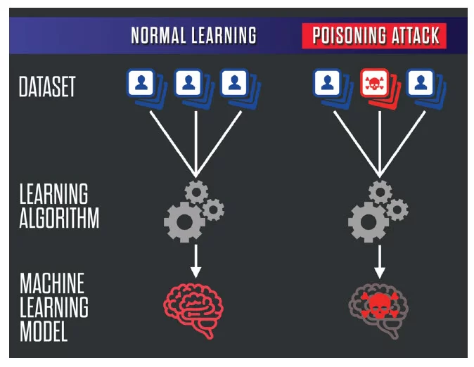
Modifying training data labels: One of the most straightforward mechanisms of data poisoning is modifying the training data labels. In this approach, the attacker selectively changes the labels of a subset of the training samples to mislead the model’s learning process as shown in Figure 17.23. For example, in a binary classification task, the attacker might flip the labels of some positive samples to negative, or vice versa. By introducing such label noise, the attacker degrades the model’s performance or cause it to make incorrect predictions for specific target instances.
Altering feature values in training data: Another mechanism of data poisoning involves altering the feature values of the training samples without modifying the labels. The attacker carefully crafts the feature values to introduce specific biases or vulnerabilities into the model. For instance, in an image classification task, the attacker might add imperceptible perturbations to a subset of images, causing the model to learn a particular pattern or association. This type of poisoning can create backdoors or trojans in the trained model, which specific input patterns can trigger.
Injecting carefully crafted malicious samples: In this mechanism, the attacker creates malicious samples designed to poison the model. These samples are crafted to have a specific impact on the model’s behavior while blending in with the legitimate training data. The attacker might use techniques such as adversarial perturbations or data synthesis to generate poisoned samples that are difficult to detect. The attacker manipulates the model’s decision boundaries by injecting these malicious samples into the training data or introducing targeted misclassifications.
Exploiting data collection and preprocessing vulnerabilities: Data poisoning attacks can also exploit the data collection and preprocessing pipeline vulnerabilities. If the data collection process is not secure or there are weaknesses in the data preprocessing steps, an attacker can manipulate the data before it reaches the training phase. For example, if data is collected from untrusted sources or issues in data cleaning or aggregation, an attacker can introduce poisoned samples or manipulate the data to their advantage.
Manipulating data at the source (e.g., sensor data): In some cases, attackers can manipulate the data at its source, such as sensor data or input devices. By tampering with the sensors or manipulating the environment in which data is collected, attackers can introduce poisoned samples or bias the data distribution. For instance, in a self-driving car scenario, an attacker might manipulate the sensors or the environment to feed misleading information into the training data, compromising the model’s ability to make safe and reliable decisions.
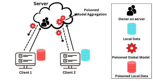
Poisoning data in online learning scenarios: Data poisoning attacks can also target ML systems that employ online learning, where the model is continuously updated with new data in real time. In such scenarios, an attacker can gradually inject poisoned samples over time, slowly manipulating the model’s behavior. Online learning systems are particularly vulnerable to data poisoning because they adapt to new data without extensive validation, making it easier for attackers to introduce malicious samples, as shown in Figure 17.24.
Collaborating with insiders to manipulate data: Sometimes, data poisoning attacks can involve collaboration with insiders with access to the training data. Malicious insiders, such as employees or data providers, can manipulate the data before it is used to train the model. Insider threats are particularly challenging to detect and prevent, as the attackers have legitimate access to the data and can carefully craft the poisoning strategy to evade detection.
These are the key mechanisms of data poisoning in ML systems. Attackers often employ these mechanisms to make their attacks more effective and harder to detect. The risk of data poisoning attacks grows as ML systems become increasingly complex and rely on larger datasets from diverse sources. Defending against data poisoning requires a multifaceted approach. ML practitioners and system designers must be aware of the various mechanisms of data poisoning and adopt a comprehensive approach to data security and model resilience. This includes secure data collection, robust data validation, and continuous model performance monitoring. Implementing secure data collection and preprocessing practices is crucial to prevent data poisoning at the source. Data validation and anomaly detection techniques can also help identify and mitigate potential poisoning attempts. Monitoring model performance for signs of data poisoning is also essential to detect and respond to attacks promptly.
Impact on ML Systems
Data poisoning attacks can severely affect ML systems, compromising their performance, reliability, and trustworthiness. The impact of data poisoning can manifest in various ways, depending on the attacker’s objectives and the specific mechanism used. Let’s explore each of the potential impacts in detail.
Degradation of model performance: One of the primary impacts of data poisoning is the degradation of the model’s overall performance. By manipulating the training data, attackers can introduce noise, biases, or inconsistencies that hinder the model’s ability to learn accurate patterns and make reliable predictions. This can reduce accuracy, precision, recall, or other performance metrics. The degradation of model performance can have significant consequences, especially in critical applications such as healthcare, finance, or security, where the reliability of predictions is crucial.
Misclassification of specific targets: Data poisoning attacks can also be designed to cause the model to misclassify specific target instances. Attackers may introduce carefully crafted poisoned samples similar to the target instances, leading the model to learn incorrect associations. This can result in the model consistently misclassifying the targeted instances, even if it performs well on other inputs. Such targeted misclassification can have severe consequences, such as causing a malware detection system to overlook specific malicious files or leading to the wrong diagnosis in a medical imaging application.
Backdoors and trojans in trained models: Data poisoning can introduce backdoors or trojans into the trained model. Backdoors are hidden functionalities that allow attackers to trigger specific behaviors or bypass normal authentication mechanisms. On the other hand, Trojans are malicious components embedded within the model that can activate specific input patterns. By poisoning the training data, attackers can create models that appear to perform normally but contain hidden vulnerabilities that can be exploited later. Backdoors and trojans can compromise the integrity and security of the ML system, allowing attackers to gain unauthorized access, manipulate predictions, or exfiltrate sensitive information.
Biased or unfair model outcomes: Data poisoning attacks can introduce biases or unfairness into the model’s predictions. By manipulating the training data distribution or injecting samples with specific biases, attackers can cause the model to learn and perpetuate discriminatory patterns. This can lead to unfair treatment of certain groups or individuals based on sensitive attributes such as race, gender, or age. Biased models can have severe societal implications, reinforcing existing inequalities and discriminatory practices. Ensuring fairness and mitigating biases is crucial for building trustworthy and ethical ML systems.
Increased false positives or false negatives: Data poisoning can also impact the model’s ability to correctly identify positive or negative instances, leading to increased false positives or false negatives. False positives occur when the model incorrectly identifies a negative instance as positive, while false negatives happen when a positive instance is misclassified as negative. The consequences of increased false positives or false negatives can be significant depending on the application. For example, in a fraud detection system, high false positives can lead to unnecessary investigations and customer frustration, while high false negatives can allow fraudulent activities to go undetected.
Compromised system reliability and trustworthiness: Data poisoning attacks can undermine ML systems’ overall reliability and trustworthiness. When models are trained on poisoned data, their predictions become unreliable and untrustworthy. This can erode user confidence in the system and lead to a loss of trust in the decisions made by the model. In critical applications where ML systems are relied upon for decision-making, such as autonomous vehicles or medical diagnosis, compromised reliability can have severe consequences, putting lives and property at risk.
Addressing the impact of data poisoning requires a proactive approach to data security, model testing, and monitoring. Organizations must implement robust measures to ensure the integrity and quality of training data, employ techniques to detect and mitigate poisoning attempts, and continuously monitor the performance and behavior of deployed models. Collaboration between ML practitioners, security experts, and domain specialists is essential to develop comprehensive strategies for preventing and responding to data poisoning attacks.
Case Study

Interestingly enough, data poisoning attacks are not always malicious (Shan et al. 2023). Nightshade, a tool developed by a team led by Professor Ben Zhao at the University of Chicago, utilizes data poisoning to help artists protect their art against scraping and copyright violations by generative AI models. Artists can use the tool to make subtle modifications to their images before uploading them online, as shown in Figure 17.25.
While these changes are indiscernible to the human eye, they can significantly disrupt the performance of generative AI models when incorporated into the training data. Generative models can be manipulated to generate hallucinations and weird images. For example, with only 300 poisoned images, the University of Chicago researchers could trick the latest Stable Diffusion model into generating images of dogs that look like cats or images of cows when prompted for cars.
As the number of poisoned images on the internet increases, the performance of the models that use scraped data will deteriorate exponentially. First, the poisoned data is hard to detect and requires manual elimination. Second, the “poison” spreads quickly to other labels because generative models rely on connections between words and concepts as they generate images. So a poisoned image of a “car” could spread into generated images associated with words like “truck,” “train,” ” bus,” etc.
On the other hand, this tool can be used maliciously and can affect legitimate applications of the generative models. This shows the very challenging and novel nature of machine learning attacks.
Figure 17.26 demonstrates the effects of different levels of data poisoning (50 samples, 100 samples, and 300 samples of poisoned images) on generating images in different categories. Notice how the images start deforming and deviating from the desired category. For example, after 300 poison samples, a car prompt generates a cow.
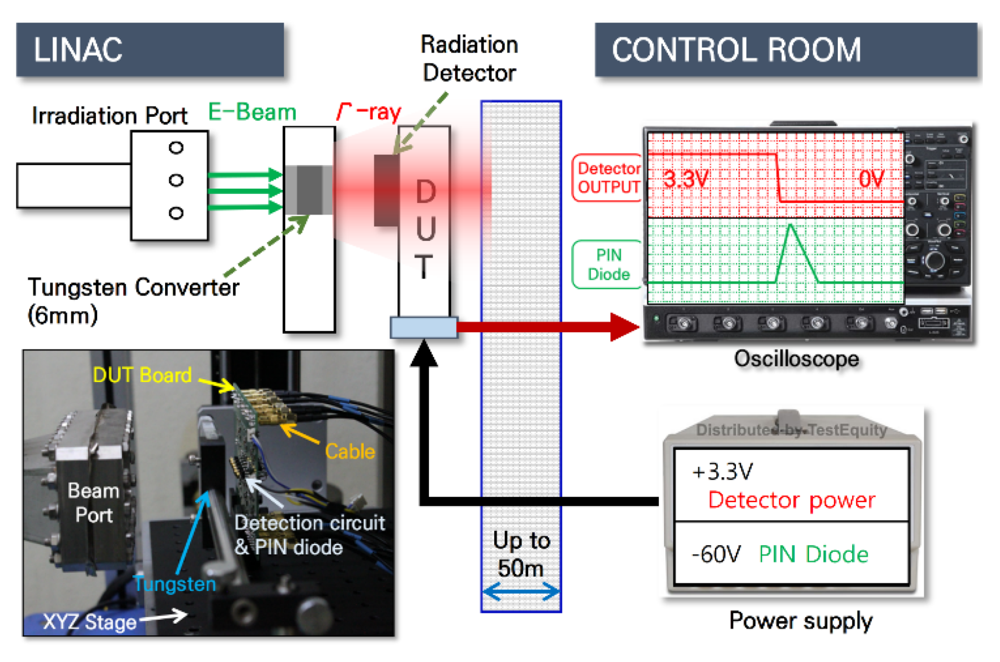
Get ready to explore the dark side of AI security! In this Colab, you’ll learn about data poisoning – how bad data can trick AI models into making wrong decisions. We’ll focus on a real-world attack against a Support Vector Machine (SVM), observing how the AI’s behavior changes under attack. This hands-on exercise will highlight why protecting AI systems is crucial, especially as they become more integrated into our lives. Think like a hacker, understand the vulnerability, and brainstorm how to defend our AI systems!
![]()
17.4.3 Distribution Shifts
Definition and Characteristics
Distribution shift refers to the phenomenon where the data distribution encountered by an ML model during deployment (inference) differs from the distribution it was trained on, as shown in Figure 17.27. This is not so much an attack as it is that the model’s robustness will vary over time. In other words, the data’s statistical properties, patterns, or underlying assumptions can change between the training and test phases.
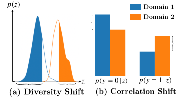
The key characteristics of distribution shift include:
Domain mismatch: The input data during inference comes from a different domain or distribution than the training data. When the input data during inference comes from a domain or distribution different from the training data, it can significantly affect the model’s performance. This is because the model has learned patterns and relationships specific to the training domain, and when applied to a different domain, those learned patterns may not hold. For example, consider a sentiment analysis model trained on movie reviews. Suppose this model is applied to analyze sentiment in tweets. In that case, it may need help to accurately classify the sentiment because the language, grammar, and context of tweets can differ from movie reviews. This domain mismatch can result in poor performance and unreliable predictions, limiting the model’s practical utility.
Temporal drift: The data distribution evolves, leading to a gradual or sudden shift in the input characteristics. Temporal drift is important because ML models are often deployed in dynamic environments where the data distribution can change over time. If the model is not updated or adapted to these changes, its performance can gradually degrade. For instance, the patterns and behaviors associated with fraudulent activities may evolve in a fraud detection system as fraudsters adapt their techniques. If the model is not retrained or updated to capture these new patterns, it may fail to detect new types of fraud effectively. Temporal drift can lead to a decline in the model’s accuracy and reliability over time, making monitoring and addressing this type of distribution shift crucial.
Contextual changes: The ML model’s context can vary, resulting in different data distributions based on factors such as location, user behavior, or environmental conditions. Contextual changes matter because ML models are often deployed in various contexts or environments that can have different data distributions. If the model cannot generalize well to these different contexts, its performance may deteriorate. For example, consider a computer vision model trained to recognize objects in a controlled lab environment. When deployed in a real-world setting, factors such as lighting conditions, camera angles, or background clutter can vary significantly, leading to a distribution shift. If the model is robust to these contextual changes, it may be able to accurately recognize objects in the new environment, limiting its practical utility.
Unrepresentative training data: The training data may only partially capture the variability and diversity of the real-world data encountered during deployment. Unrepresentative training data can lead to biased or skewed models that perform poorly on real-world data. Suppose the training data needs to capture the variability and diversity of the real-world data adequately. In that case, the model may learn patterns specific to the training set but needs to generalize better to new, unseen data. This can result in poor performance, biased predictions, and limited model applicability. For instance, if a facial recognition model is trained primarily on images of individuals from a specific demographic group, it may struggle to accurately recognize faces from other demographic groups when deployed in a real-world setting. Ensuring that the training data is representative and diverse is crucial for building models that can generalize well to real-world scenarios.
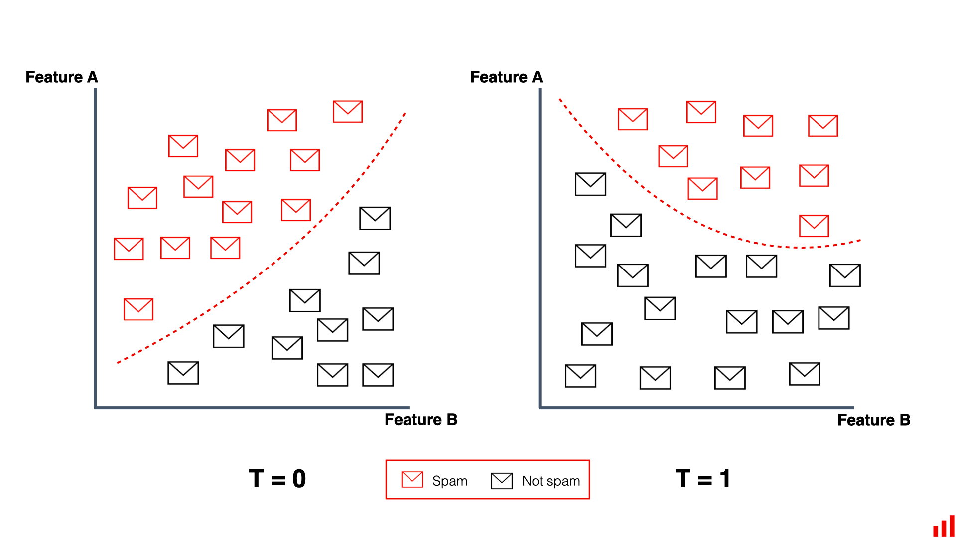
Distribution shift can manifest in various forms, such as:
Covariate shift: The distribution of the input features (covariates) changes while the conditional distribution of the target variable given the input remains the same. Covariate shift matters because it can impact the model’s ability to make accurate predictions when the input features (covariates) differ between the training and test data. Even if the relationship between the input features and the target variable remains the same, a change in the distribution of the input features can affect the model’s performance. For example, consider a model trained to predict housing prices based on features like square footage, number of bedrooms, and location. Suppose the distribution of these features in the test data significantly differs from the training data (e.g., the test data contains houses with much larger square footage). In that case, the model’s predictions may become less accurate. Addressing covariate shifts is important to ensure the model’s robustness and reliability when applied to new data.
Concept drift: The relationship between the input features and the target variable changes over time, altering the underlying concept the model is trying to learn, as shown in Figure 17.28. Concept drift is important because it indicates changes in the fundamental relationship between the input features and the target variable over time. When the underlying concept that the model is trying to learn shifts, its performance can deteriorate if not adapted to the new concept. For instance, in a customer churn prediction model, the factors influencing customer churn may evolve due to market conditions, competitor offerings, or customer preferences. If the model is not updated to capture these changes, its predictions may become less accurate and irrelevant. Detecting and adapting to concept drift is crucial to maintaining the model’s effectiveness and alignment with evolving real-world concepts.
Domain generalization: The model must generalize to unseen domains or distributions not present during training. Domain generalization is important because it enables ML models to be applied to new, unseen domains without requiring extensive retraining or adaptation. In real-world scenarios, training data that covers all possible domains or distributions that the model may encounter is often infeasible. Domain generalization techniques aim to learn domain-invariant features or models that can generalize well to new domains. For example, consider a model trained to classify images of animals. If the model can learn features invariant to different backgrounds, lighting conditions, or poses, it can generalize well to classify animals in new, unseen environments. Domain generalization is crucial for building models that can be deployed in diverse and evolving real-world settings.
The presence of a distribution shift can significantly impact the performance and reliability of ML models, as the models may need help generalizing well to the new data distribution. Detecting and adapting to distribution shifts is crucial to ensure ML systems’ robustness and practical utility in real-world scenarios.
Mechanisms of Distribution Shifts
The mechanisms of distribution shift, such as changes in data sources, temporal evolution, domain-specific variations, selection bias, feedback loops, and adversarial manipulations, are important to understand because they help identify the underlying causes of distribution shift. By understanding these mechanisms, practitioners can develop targeted strategies to mitigate their impact and improve the model’s robustness. Here are some common mechanisms:

Changes in data sources: Distribution shifts can occur when the data sources used for training and inference differ. For example, if a model is trained on data from one sensor but deployed on data from another sensor with different characteristics, it can lead to a distribution shift.
Temporal evolution: Over time, the underlying data distribution can evolve due to changes in user behavior, market dynamics, or other temporal factors. For instance, in a recommendation system, user preferences may shift over time, leading to a distribution shift in the input data, as shown in Figure 17.29.
Domain-specific variations: Different domains or contexts can have distinct data distributions. A model trained on data from one domain may only generalize well to another domain with appropriate adaptation techniques. For example, an image classification model trained on indoor scenes may struggle when applied to outdoor scenes.
Selection bias: A Distribution shift can arise from selection bias during data collection or sampling. If the training data does not represent the true population or certain subgroups are over- or underrepresented, this can lead to a mismatch between the training and test distributions.
Feedback loops: In some cases, the predictions or actions taken by an ML model can influence future data distribution. For example, in a dynamic pricing system, the prices set by the model can impact customer behavior, leading to a shift in the data distribution over time.
Adversarial manipulations: Adversaries can intentionally manipulate the input data to create a distribution shift and deceive the ML model. By introducing carefully crafted perturbations or generating out-of-distribution samples, attackers can exploit the model’s vulnerabilities and cause it to make incorrect predictions.
Understanding the mechanisms of distribution shift is important for developing effective strategies to detect and mitigate its impact on ML systems. By identifying the sources and characteristics of the shift, practitioners can design appropriate techniques, such as domain adaptation, transfer learning, or continual learning, to improve the model’s robustness and performance under distributional changes.
Impact on ML Systems
Distribution shifts can significantly negatively impact the performance and reliability of ML systems. Here are some key ways in which distribution shift can affect ML models:
Degraded predictive performance: When the data distribution encountered during inference differs from the training distribution, the model’s predictive accuracy can deteriorate. The model may need help generalizing the new data well, leading to increased errors and suboptimal performance.
Reduced reliability and trustworthiness: Distribution shift can undermine the reliability and trustworthiness of ML models. If the model’s predictions become unreliable or inconsistent due to the shift, users may lose confidence in the system’s outputs, leading to potential misuse or disuse of the model.
Biased predictions: Distribution shift can introduce biases in the model’s predictions. If the training data does not represent the real-world distribution or certain subgroups are underrepresented, the model may make biased predictions that discriminate against certain groups or perpetuate societal biases.
Increased uncertainty and risk: Distribution shift introduces additional uncertainty and risk into the ML system. The model’s behavior and performance may become less predictable, making it challenging to assess its reliability and suitability for critical applications. This uncertainty can lead to increased operational risks and potential failures.
Adaptability challenges: ML models trained on a specific data distribution may need help to adapt to changing environments or new domains. The lack of adaptability can limit the model’s usefulness and applicability in dynamic real-world scenarios where the data distribution evolves.
Maintenance and update difficulties: Distribution shift can complicate the maintenance and updating of ML models. As the data distribution changes, the model may require frequent retraining or fine-tuning to maintain its performance. This can be time-consuming and resource-intensive, especially if the shift occurs rapidly or continuously.
Vulnerability to adversarial attacks: Distribution shift can make ML models more vulnerable to adversarial attacks. Adversaries can exploit the model’s sensitivity to distributional changes by crafting adversarial examples outside the training distribution, causing the model to make incorrect predictions or behave unexpectedly.
To mitigate the impact of distribution shifts, it is crucial to develop robust ML systems that detect and adapt to distributional changes. Techniques such as domain adaptation, transfer learning, and continual learning can help improve the model’s generalization ability across different distributions. ML model monitoring, testing, and updating are also necessary to ensure their performance and reliability during distribution shifts.
17.4.4 Detection and Mitigation
Adversarial Attacks
As you may recall from above, adversarial attacks pose a significant threat to the robustness and reliability of ML systems. These attacks involve crafting carefully designed inputs, known as adversarial examples, to deceive ML models and cause them to make incorrect predictions. To safeguard ML systems against adversarial attacks, developing effective techniques for detecting and mitigating these threats is crucial.
Adversarial Example Detection Techniques
Detecting adversarial examples is the first line of defense against adversarial attacks. Several techniques have been proposed to identify and flag suspicious inputs that may be adversarial.
Statistical methods aim to detect adversarial examples by analyzing the statistical properties of the input data. These methods often compare the input data distribution to a reference distribution, such as the training data distribution or a known benign distribution. Techniques like the Kolmogorov-Smirnov (Berger and Zhou 2014) test or the Anderson-Darling test can be used to measure the discrepancy between the distributions and flag inputs that deviate significantly from the expected distribution.
Kernel density estimation (KDE) is a non-parametric technique used to estimate the probability density function of a dataset. In the context of adversarial example detection, KDE can be used to estimate the density of benign examples in the input space. Adversarial examples often lie in low-density regions and can be detected by comparing their estimated density to a threshold. Inputs with an estimated density below the threshold are flagged as potential adversarial examples.
Another technique is feature squeezing (Panda, Chakraborty, and Roy 2019), which reduces the complexity of the input space by applying dimensionality reduction or discretization. The idea behind feature squeezing is that adversarial examples often rely on small, imperceptible perturbations that can be eliminated or reduced through these transformations. Inconsistencies can be detected by comparing the model’s predictions on the original input and the squeezed input, indicating the presence of adversarial examples.
Model uncertainty estimation techniques aim to quantify the confidence or uncertainty associated with a model’s predictions. Adversarial examples often exploit regions of high uncertainty in the model’s decision boundary. By estimating the uncertainty using techniques like Bayesian neural networks, dropout-based uncertainty estimation, or ensemble methods, inputs with high uncertainty can be flagged as potential adversarial examples.
Adversarial Defense Strategies
Once adversarial examples are detected, various defense strategies can be employed to mitigate their impact and improve the robustness of ML models.
Adversarial training is a technique that involves augmenting the training data with adversarial examples and retraining the model on this augmented dataset. Exposing the model to adversarial examples during training teaches it to classify them correctly and becomes more robust to adversarial attacks. Adversarial training can be performed using various attack methods, such as the Fast Gradient Sign Method (FGSM) or Projected Gradient Descent (PGD) (Madry et al. 2017).
Defensive distillation (Papernot et al. 2016) is a technique that trains a second model (the student model) to mimic the behavior of the original model (the teacher model). The student model is trained on the soft labels produced by the teacher model, which are less sensitive to small perturbations. Using the student model for inference can reduce the impact of adversarial perturbations, as the student model learns to generalize better and is less sensitive to adversarial noise.
Input preprocessing and transformation techniques aim to remove or mitigate the effect of adversarial perturbations before feeding the input to the ML model. These techniques include image denoising, JPEG compression, random resizing, padding, or applying random transformations to the input data. By reducing the impact of adversarial perturbations, these preprocessing steps can help improve the model’s robustness to adversarial attacks.
Ensemble methods combine multiple models to make more robust predictions. The ensemble can reduce the impact of adversarial attacks by using a diverse set of models with different architectures, training data, or hyperparameters. Adversarial examples that fool one model may not fool others in the ensemble, leading to more reliable and robust predictions. Model diversification techniques, such as using different preprocessing techniques or feature representations for each model in the ensemble, can further enhance the robustness.
Robustness Evaluation and Testing
Conduct thorough evaluation and testing to assess the effectiveness of adversarial defense techniques and measure the robustness of ML models.
Adversarial robustness metrics quantify the model’s resilience to adversarial attacks. These metrics can include the model’s accuracy on adversarial examples, the average distortion required to fool the model, or the model’s performance under different attack strengths. By comparing these metrics across different models or defense techniques, practitioners can assess and compare their robustness levels.
Standardized adversarial attack benchmarks and datasets provide a common ground for evaluating and comparing the robustness of ML models. These benchmarks include datasets with pre-generated adversarial examples and tools and frameworks for generating adversarial attacks. Examples of popular adversarial attack benchmarks include the MNIST-C, CIFAR-10-C, and ImageNet-C (Hendrycks and Dietterich 2019) datasets, which contain corrupted or perturbed versions of the original datasets.
Practitioners can develop more robust and resilient ML systems by leveraging these adversarial example detection techniques, defense strategies, and robustness evaluation methods. However, it is important to note that adversarial robustness is an ongoing research area, and no single technique provides complete protection against all types of adversarial attacks. A comprehensive approach that combines multiple defense mechanisms and regular testing is essential to maintain the security and reliability of ML systems in the face of evolving adversarial threats.
Data Poisoning
Recall that data poisoning is an attack that targets the integrity of the training data used to build ML models. By manipulating or corrupting the training data, attackers can influence the model’s behavior and cause it to make incorrect predictions or perform unintended actions. Detecting and mitigating data poisoning attacks is crucial to ensure the trustworthiness and reliability of ML systems, as shown in Figure 17.30.
Anomaly Detection Techniques for Identifying Poisoned Data
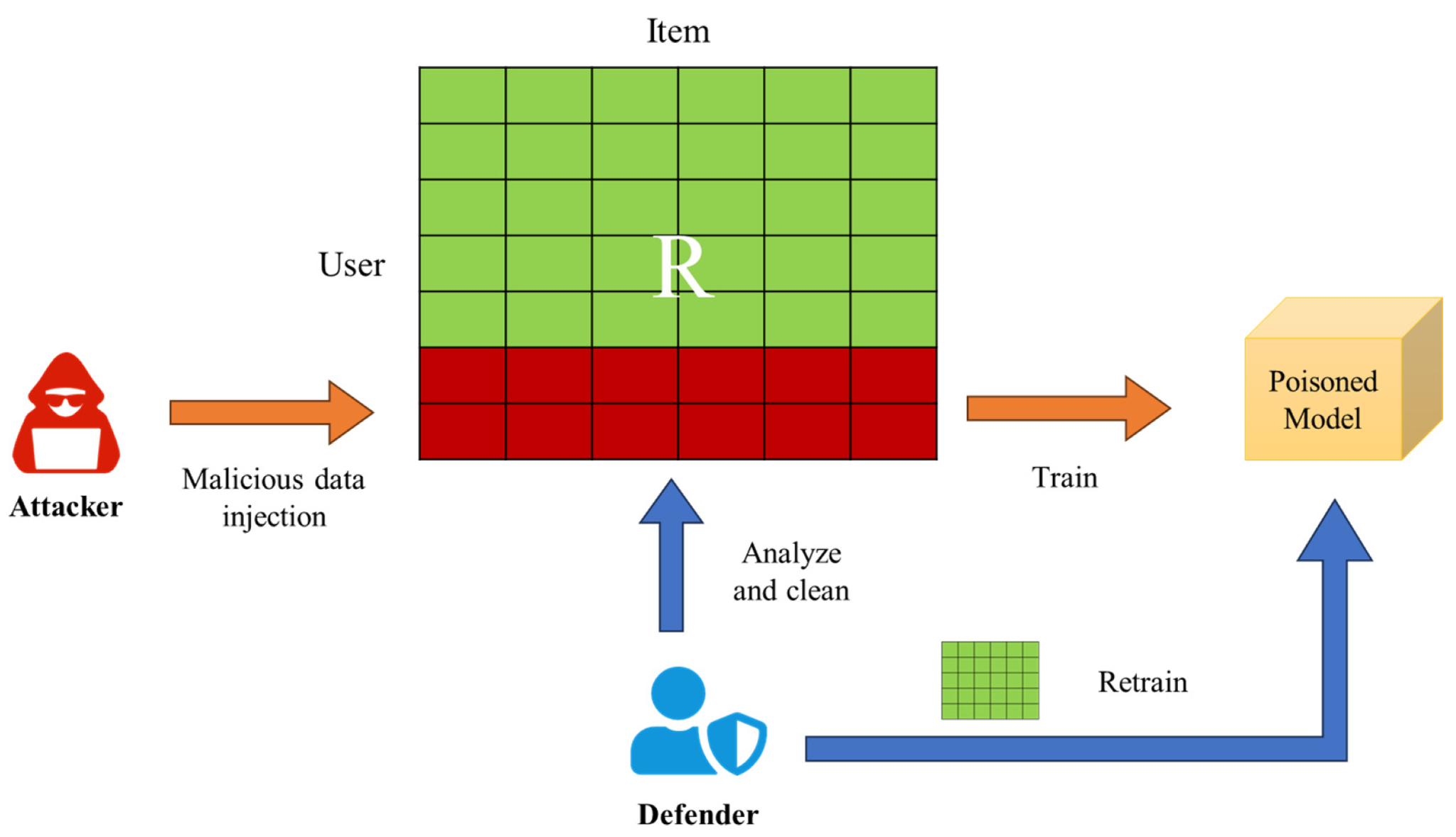
Statistical outlier detection methods identify data points that deviate significantly from most data. These methods assume that poisoned data instances are likely to be statistical outliers. Techniques such as the Z-score method, Tukey’s method, or the Mahalanobis distance can be used to measure the deviation of each data point from the central tendency of the dataset. Data points that exceed a predefined threshold are flagged as potential outliers and considered suspicious for data poisoning.
Clustering-based methods group similar data points together based on their features or attributes. The assumption is that poisoned data instances may form distinct clusters or lie far away from the normal data clusters. By applying clustering algorithms like K-means, DBSCAN, or hierarchical clustering, anomalous clusters or data points that do not belong to any cluster can be identified. These anomalous instances are then treated as potentially poisoned data.
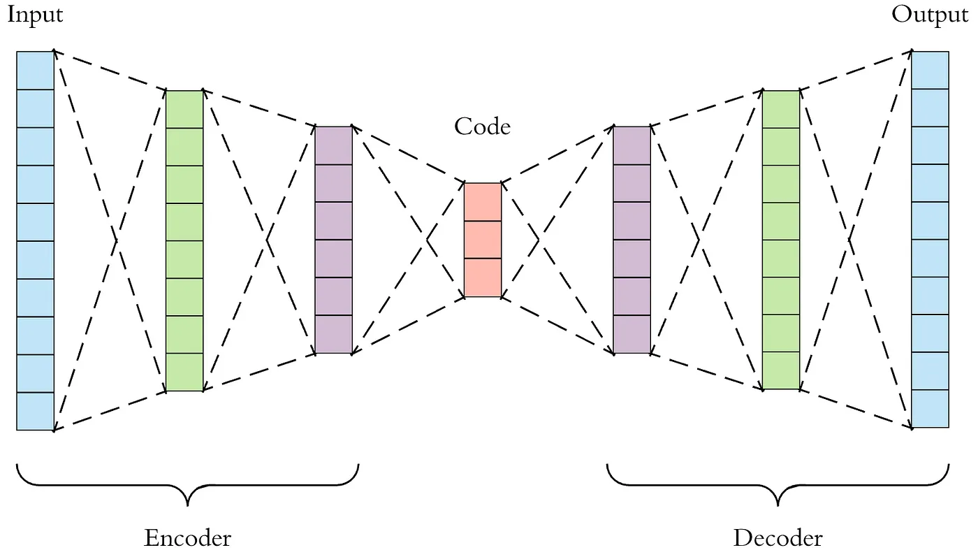
Autoencoders are neural networks trained to reconstruct the input data from a compressed representation, as shown in Figure 17.31. They can be used for anomaly detection by learning the normal patterns in the data and identifying instances that deviate from them. During training, the autoencoder is trained on clean, unpoisoned data. At inference time, the reconstruction error for each data point is computed. Data points with high reconstruction errors are considered abnormal and potentially poisoned, as they do not conform to the learned normal patterns.
Data Sanitization and Preprocessing Techniques
Data poisoning can be avoided by cleaning data, which involves identifying and removing or correcting noisy, incomplete, or inconsistent data points. Techniques such as data deduplication, missing value imputation, and outlier removal can be applied to improve the quality of the training data. By eliminating or filtering out suspicious or anomalous data points, the impact of poisoned instances can be reduced.
Data validation involves verifying the integrity and consistency of the training data. This can include checking for data type consistency, range validation, and cross-field dependencies. By defining and enforcing data validation rules, anomalous or inconsistent data points indicative of data poisoning can be identified and flagged for further investigation.
Data provenance and lineage tracking involve maintaining a record of data’s origin, transformations, and movements throughout the ML pipeline. By documenting the data sources, preprocessing steps, and any modifications made to the data, practitioners can trace anomalies or suspicious patterns back to their origin. This helps identify potential points of data poisoning and facilitates the investigation and mitigation process.
Robust Training Techniques
Robust optimization techniques can be used to modify the training objective to minimize the impact of outliers or poisoned instances. This can be achieved by using robust loss functions less sensitive to extreme values, such as the Huber loss or the modified Huber loss. Regularization techniques, such as L1 or L2 regularization, can also help in reducing the model’s sensitivity to poisoned data by constraining the model’s complexity and preventing overfitting.
Robust loss functions are designed to be less sensitive to outliers or noisy data points. Examples include the modified Huber loss, the Tukey loss (Beaton and Tukey 1974), and the trimmed mean loss. These loss functions down-weight or ignore the contribution of abnormal instances during training, reducing their impact on the model’s learning process. Robust objective functions, such as the minimax or distributionally robust objective, aim to optimize the model’s performance under worst-case scenarios or in the presence of adversarial perturbations.
Data augmentation techniques involve generating additional training examples by applying random transformations or perturbations to the existing data Figure 17.32. This helps in increasing the diversity and robustness of the training dataset. By introducing controlled variations in the data, the model becomes less sensitive to specific patterns or artifacts that may be present in poisoned instances. Randomization techniques, such as random subsampling or bootstrap aggregating, can also help reduce the impact of poisoned data by training multiple models on different subsets of the data and combining their predictions.

Secure and Trusted Data Sourcing
Implementing the best data collection and curation practices can help mitigate the risk of data poisoning. This includes establishing clear data collection protocols, verifying the authenticity and reliability of data sources, and conducting regular data quality assessments. Sourcing data from trusted and reputable providers and following secure data handling practices can reduce the likelihood of introducing poisoned data into the training pipeline.
Strong data governance and access control mechanisms are essential to prevent unauthorized modifications or tampering with the training data. This involves defining clear roles and responsibilities for data access, implementing access control policies based on the principle of least privilege, and monitoring and logging data access activities. By restricting access to the training data and maintaining an audit trail, potential data poisoning attempts can be detected and investigated.
Detecting and mitigating data poisoning attacks requires a multifaceted approach that combines anomaly detection, data sanitization, robust training techniques, and secure data sourcing practices. By implementing these measures, ML practitioners can improve the resilience of their models against data poisoning and ensure the integrity and trustworthiness of the training data. However, it is important to note that data poisoning is an active area of research, and new attack vectors and defense mechanisms continue to emerge. Staying informed about the latest developments and adopting a proactive and adaptive approach to data security is crucial for maintaining the robustness of ML systems.
Distribution Shifts
Detecting and Mitigating Distribution Shifts
Recall that distribution shifts occur when the data distribution encountered by a machine learning (ML) model during deployment differs from the distribution it was trained on. These shifts can significantly impact the model’s performance and generalization ability, leading to suboptimal or incorrect predictions. Detecting and mitigating distribution shifts is crucial to ensure the robustness and reliability of ML systems in real-world scenarios.
Detection Techniques for Distribution Shifts
Statistical tests can be used to compare the distributions of the training and test data to identify significant differences. Techniques such as the Kolmogorov-Smirnov test or the Anderson-Darling test measure the discrepancy between two distributions and provide a quantitative assessment of the presence of distribution shift. By applying these tests to the input features or the model’s predictions, practitioners can detect if there is a statistically significant difference between the training and test distributions.
Divergence metrics quantify the dissimilarity between two probability distributions. Commonly used divergence metrics include the Kullback-Leibler (KL) divergence and the Jensen-Shannon (JS) divergence. By calculating the divergence between the training and test data distributions, practitioners can assess the extent of the distribution shift. High divergence values indicate a significant difference between the distributions, suggesting the presence of a distribution shift.
Uncertainty quantification techniques, such as Bayesian neural networks or ensemble methods, can estimate the uncertainty associated with the model’s predictions. When a model is applied to data from a different distribution, its predictions may have higher uncertainty. By monitoring the uncertainty levels, practitioners can detect distribution shifts. If the uncertainty consistently exceeds a predetermined threshold for test samples, it suggests that the model is operating outside its trained distribution.
In addition, domain classifiers are trained to distinguish between different domains or distributions. Practitioners can detect distribution shifts by training a classifier to differentiate between the training and test domains. If the domain classifier achieves high accuracy in distinguishing between the two domains, it indicates a significant difference in the underlying distributions. The performance of the domain classifier serves as a measure of the distribution shift.
Mitigation Techniques for Distribution Shifts
Transfer learning leverages knowledge gained from one domain to improve performance in another, as shown in Figure 17.33. By using pre-trained models or transferring learned features from a source domain to a target domain, transfer learning can help mitigate the impact of distribution shifts. The pre-trained model can be fine-tuned on a small amount of labeled data from the target domain, allowing it to adapt to the new distribution. Transfer learning is particularly effective when the source and target domains share similar characteristics or when labeled data in the target domain is scarce.
Continual learning, also known as lifelong learning, enables ML models to learn continuously from new data distributions while retaining knowledge from previous distributions. Techniques such as elastic weight consolidation (EWC) (Kirkpatrick et al. 2017) or gradient episodic memory (GEM) (Lopez-Paz and Ranzato 2017) allow models to adapt to evolving data distributions over time. These techniques aim to balance the plasticity of the model (ability to learn from new data) with the stability of the model (retaining previously learned knowledge). By incrementally updating the model with new data and mitigating catastrophic forgetting, continual learning helps models stay robust to distribution shifts.
Data augmentation techniques, such as those we have seen previously, involve applying transformations or perturbations to the existing training data to increase its diversity and improve the model’s robustness to distribution shifts. By introducing variations in the data, such as rotations, translations, scaling, or adding noise, data augmentation helps the model learn invariant features and generalize better to unseen distributions. Data augmentation can be performed during training and inference to improve the model’s ability to handle distribution shifts.
Ensemble methods combine multiple models to make predictions more robust to distribution shifts. By training models on different subsets of the data, using different algorithms, or with different hyperparameters, ensemble methods can capture diverse aspects of the data distribution. When presented with a shifted distribution, the ensemble can leverage the strengths of individual models to make more accurate and stable predictions. Techniques like bagging, boosting, or stacking can create effective ensembles.
Regularly updating models with new data from the target distribution is crucial to mitigate the impact of distribution shifts. As the data distribution evolves, models should be retrained or fine-tuned on the latest available data to adapt to the changing patterns. Monitoring model performance and data characteristics can help detect when an update is necessary. By keeping the models up to date, practitioners can ensure they remain relevant and accurate in the face of distribution shifts.
Evaluating models using robust metrics less sensitive to distribution shifts can provide a more reliable assessment of model performance. Metrics such as the area under the precision-recall curve (AUPRC) or the F1 score are more robust to class imbalance and can better capture the model’s performance across different distributions. Additionally, using domain-specific evaluation metrics that align with the desired outcomes in the target domain can provide a more meaningful measure of the model’s effectiveness.
Detecting and mitigating distribution shifts is an ongoing process that requires continuous monitoring, adaptation, and improvement. By employing a combination of detection techniques and mitigation strategies, ML practitioners can proactively identify and address distribution shifts, ensuring the robustness and reliability of their models in real-world deployments. It is important to note that distribution shifts can take various forms and may require domain-specific approaches depending on the nature of the data and the application. Staying informed about the latest research and best practices in handling distribution shifts is essential for building resilient ML systems.
17.5 Software Faults
17.5.1 Definition and Characteristics
Software faults refer to defects, errors, or bugs in the runtime software frameworks and components that support the execution and deployment of ML models (Myllyaho et al. 2022). These faults can arise from various sources, such as programming mistakes, design flaws, or compatibility issues (H. Zhang 2008), and can have significant implications for ML systems’ performance, reliability, and security. Software faults in ML frameworks exhibit several key characteristics:
Diversity: Software faults can manifest in different forms, ranging from simple logic and syntax mistakes to more complex issues like memory leaks, race conditions, and integration problems. The variety of fault types adds to the challenge of detecting and mitigating them effectively.
Propagation: In ML systems, software faults can propagate through the various layers and components of the framework. A fault in one module can trigger a cascade of errors or unexpected behavior in other parts of the system, making it difficult to pinpoint the root cause and assess the full impact of the fault.
Intermittency: Some software faults may exhibit intermittent behavior, occurring sporadically or under specific conditions. These faults can be particularly challenging to reproduce and debug, as they may manifest inconsistently during testing or normal operation.
Interaction with ML models: Software faults in ML frameworks can interact with the trained models in subtle ways. For example, a fault in the data preprocessing pipeline may introduce noise or bias into the model’s inputs, leading to degraded performance or incorrect predictions. Similarly, faults in the model serving component may cause inconsistencies between the training and inference environments.
Impact on system properties: Software faults can compromise various desirable properties of ML systems, such as performance, scalability, reliability, and security. Faults may lead to slowdowns, crashes, incorrect outputs, or vulnerabilities that attackers can exploit.
Dependency on external factors: The occurrence and impact of software faults in ML frameworks often depend on external factors, such as the choice of hardware, operating system, libraries, and configurations. Compatibility issues and version mismatches can introduce faults that are difficult to anticipate and mitigate.
Understanding the characteristics of software faults in ML frameworks is crucial for developing effective fault prevention, detection, and mitigation strategies. By recognizing the diversity, propagation, intermittency, and impact of software faults, ML practitioners can design more robust and reliable systems resilient to these issues.
17.5.2 Mechanisms of Software Faults in ML Frameworks
Machine learning frameworks, such as TensorFlow, PyTorch, and sci-kit-learn, provide powerful tools and abstractions for building and deploying ML models. However, these frameworks are not immune to software faults that can impact ML systems’ performance, reliability, and correctness. Let’s explore some of the common software faults that can occur in ML frameworks:
Memory Leaks and Resource Management Issues: Improper memory management, such as failing to release memory or close file handles, can lead to memory leaks and resource exhaustion over time. This issue is compounded by inefficient memory usage, where creating unnecessary copies of large tensors or not leveraging memory-efficient data structures can cause excessive memory consumption and degrade system performance. Additionally, failing to manage GPU memory properly can result in out-of-memory errors or suboptimal utilization of GPU resources, further exacerbating the problem as shown in Figure 17.34.
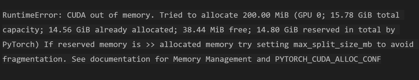
Synchronization and Concurrency Problems: Incorrect synchronization between threads or processes can lead to race conditions, deadlocks, or inconsistent behavior in multi-threaded or distributed ML systems. This issue is often tied to improper handling of asynchronous operations, such as non-blocking I/O or parallel data loading, which can cause synchronization issues and impact the correctness of the ML pipeline. Moreover, proper coordination and communication between distributed nodes in a cluster can result in consistency or stale data during training or inference, compromising the reliability of the ML system.
Compatibility Issues: Mismatches between the versions of ML frameworks, libraries, or dependencies can introduce compatibility problems and runtime errors. Upgrading or changing the versions of underlying libraries without thoroughly testing the impact on the ML system can lead to unexpected behavior or breakages. Furthermore, inconsistencies between the training and deployment environments, such as differences in hardware, operating systems, or package versions, can cause compatibility issues and affect the reproducibility of ML models, making it challenging to ensure consistent performance across different platforms.
Numerical Instability and Precision Errors: Inadequate handling of numerical instabilities, such as division by zero, underflow, or overflow, can lead to incorrect calculations or convergence issues during training. This problem is compounded by insufficient precision or rounding errors, which can accumulate over time and impact the accuracy of the ML models, especially in deep learning architectures with many layers. Moreover, improper scaling or normalization of input data can cause numerical instabilities and affect the convergence and performance of optimization algorithms, resulting in suboptimal or unreliable model performance.
Inadequate Error Handling and Exception Management: Proper error handling and exception management can prevent ML systems from crashing or behaving unexpectedly when encountering exceptional conditions or invalid inputs. Failing to catch and handle specific exceptions or relying on generic exception handling can make it difficult to diagnose and recover from errors gracefully, leading to system instability and reduced reliability. Furthermore, incomplete or misleading error messages can hinder the ability to effectively debug and resolve software faults in ML frameworks, prolonging the time required to identify and fix issues.
17.5.3 Impact on ML Systems
Software faults in machine learning frameworks can have significant and far-reaching impacts on ML systems’ performance, reliability, and security. Let’s explore the various ways in which software faults can affect ML systems:
Performance Degradation and System Slowdowns: Memory leaks and inefficient resource management can lead to gradual performance degradation over time as the system becomes increasingly memory-constrained and spends more time on garbage collection or memory swapping (Maas et al. 2024). This issue is compounded by synchronization issues and concurrency bugs, which can cause delays, reduced throughput, and suboptimal utilization of computational resources, especially in multi-threaded or distributed ML systems. Furthermore, compatibility problems or inefficient code paths can introduce additional overhead and slowdowns, affecting the overall performance of the ML system.
Incorrect Predictions or Outputs: Software faults in data preprocessing, feature engineering, or model evaluation can introduce biases, noise, or errors propagating through the ML pipeline and resulting in incorrect predictions or outputs. Over time, numerical instabilities, precision errors, or rounding issues can accumulate and lead to degraded accuracy or convergence problems in the trained models. Moreover, faults in the model serving or inference components can cause inconsistencies between the expected and actual outputs, leading to incorrect or unreliable predictions in production.
Reliability and Stability Issues: Software faults can cause Unparalleled exceptions, crashes, or sudden terminations that can compromise the reliability and stability of ML systems, especially in production environments. Intermittent or sporadic faults can be difficult to reproduce and diagnose, leading to unpredictable behavior and reduced confidence in the ML system’s outputs. Additionally, faults in checkpointing, model serialization, or state management can cause data loss or inconsistencies, affecting the reliability and recoverability of the ML system.
Security Vulnerabilities: Software faults, such as buffer overflows, injection vulnerabilities, or improper access control, can introduce security risks and expose the ML system to potential attacks or unauthorized access. Adversaries may exploit faults in the preprocessing or feature extraction stages to manipulate the input data and deceive the ML models, leading to incorrect or malicious behavior. Furthermore, inadequate protection of sensitive data, such as user information or confidential model parameters, can lead to data breaches or privacy violations (Q. Li et al. 2023).
Difficulty in Reproducing and Debugging: Software faults can make it challenging to reproduce and debug issues in ML systems, especially when the faults are intermittent or dependent on specific runtime conditions. Incomplete or ambiguous error messages, coupled with the complexity of ML frameworks and models, can prolong the debugging process and hinder the ability to identify and fix the underlying faults. Moreover, inconsistencies between development, testing, and production environments can make reproducing and diagnosing faults in specific contexts difficult.
Increased Development and Maintenance Costs Software faults can lead to increased development and maintenance costs, as teams spend more time and resources debugging, fixing, and validating the ML system. The need for extensive testing, monitoring, and fault-tolerant mechanisms to mitigate the impact of software faults can add complexity and overhead to the ML development process. Frequent patches, updates, and bug fixes to address software faults can disrupt the development workflow and require additional effort to ensure the stability and compatibility of the ML system.
Understanding the potential impact of software faults on ML systems is crucial for prioritizing testing efforts, implementing fault-tolerant designs, and establishing effective monitoring and debugging practices. By proactively addressing software faults and their consequences, ML practitioners can build more robust, reliable, and secure ML systems that deliver accurate and trustworthy results.
17.5.4 Detection and Mitigation
Detecting and mitigating software faults in machine learning frameworks is essential to ensure ML systems’ reliability, performance, and security. Let’s explore various techniques and approaches that can be employed to identify and address software faults effectively:
Thorough Testing and Validation: Comprehensive unit testing of individual components and modules can verify their correctness and identify potential faults early in development. Integration testing validates the interaction and compatibility between different components of the ML framework, ensuring seamless integration. Systematic testing of edge cases, boundary conditions, and exceptional scenarios helps uncover hidden faults and vulnerabilities. Continuous testing and regression testing as shown in Figure 17.35 detect faults introduced by code changes or updates to the ML framework.
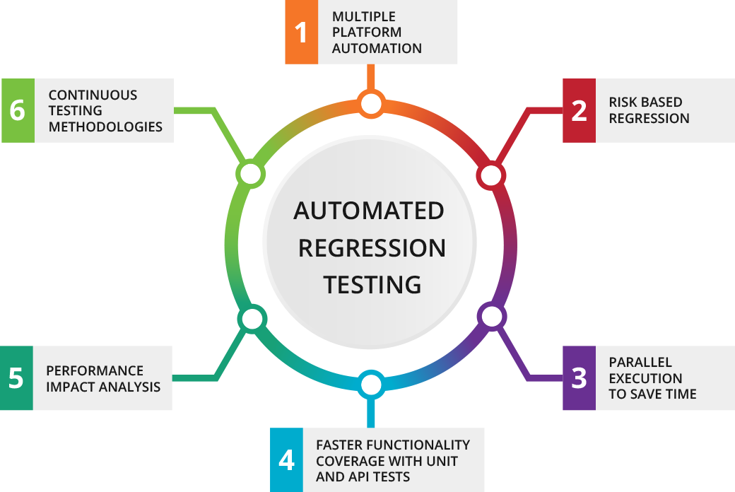
Static Code Analysis and Linting: Utilizing static code analysis tools automatically identifies potential coding issues, such as syntax errors, undefined variables, or security vulnerabilities. Enforcing coding standards and best practices through linting tools maintains code quality and reduces the likelihood of common programming mistakes. Conducting regular code reviews allows manual inspection of the codebase, identification of potential faults, and ensures adherence to coding guidelines and design principles.
Runtime Monitoring and Logging: Implementing comprehensive logging mechanisms captures relevant information during runtime, such as input data, model parameters, and system events. Monitoring key performance metrics, resource utilization, and error rates helps detect anomalies, performance bottlenecks, or unexpected behavior. Employing runtime assertion checks and invariants validates assumptions and detects violations of expected conditions during program execution. Utilizing profiling tools identifies performance bottlenecks, memory leaks, or inefficient code paths that may indicate the presence of software faults.
Fault-Tolerant Design Patterns: Implementing error handling and exception management mechanisms enables graceful handling and recovery from exceptional conditions or runtime errors. Employing redundancy and failover mechanisms, such as backup systems or redundant computations, ensures the availability and reliability of the ML system in the presence of faults. Designing modular and loosely coupled architectures minimizes the propagation and impact of faults across different components of the ML system. Utilizing checkpointing and recovery mechanisms (Eisenman et al. 2022) allows the system to resume from a known stable state in case of failures or interruptions.
Regular Updates and Patches: Staying up to date with the latest versions and patches of the ML frameworks, libraries, and dependencies provides benefits from bug fixes, security updates, and performance improvements. Monitoring release notes, security advisories, and community forums inform practitioners about known issues, vulnerabilities, or compatibility problems in the ML framework. Establishing a systematic process for testing and validating updates and patches before applying them to production systems ensures stability and compatibility.
Containerization and Isolation: Leveraging containerization technologies, such as Docker or Kubernetes, encapsulates ML components and their dependencies in isolated environments. Utilizing containerization ensures consistent and reproducible runtime environments across development, testing, and production stages, reducing the likelihood of compatibility issues or environment-specific faults. Employing isolation techniques, such as virtual environments or sandboxing, prevents faults or vulnerabilities in one component from affecting other parts of the ML system.
Automated Testing and Continuous Integration/Continuous Deployment (CI/CD): Implement automated testing frameworks and scripts, execute comprehensive test suites, and catch faults early in development. Integrating automated testing into the CI/CD pipeline, as shown in Figure 17.36, ensures that code changes are thoroughly tested before being merged or deployed to production. Utilizing continuous monitoring and automated alerting systems detects and notifies developers and operators about potential faults or anomalies in real-time.
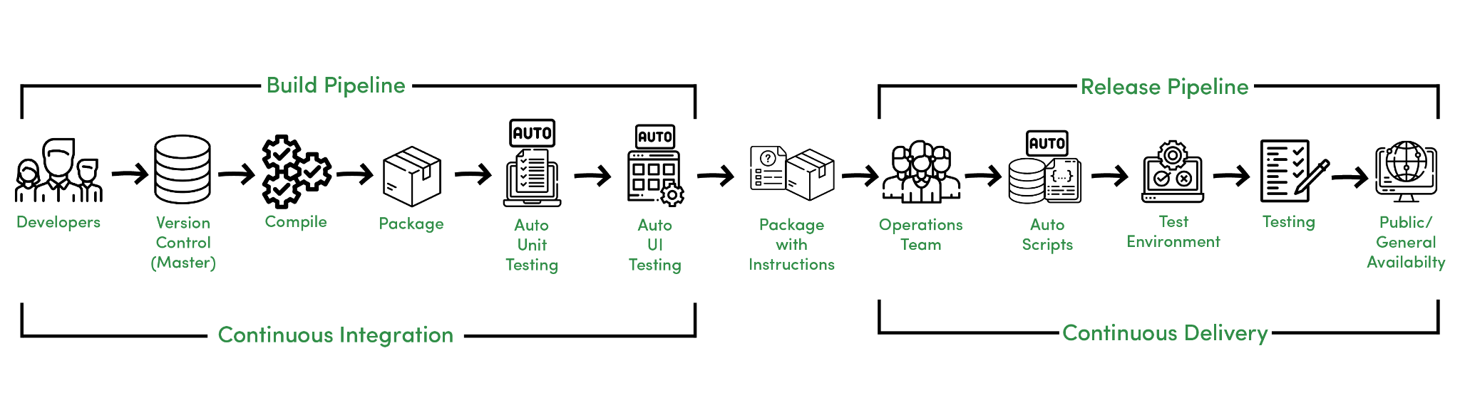
Adopting a proactive and systematic approach to fault detection and mitigation can significantly improve ML systems’ robustness, reliability, and maintainability. By investing in comprehensive testing, monitoring, and fault-tolerant design practices, organizations can minimize the impact of software faults and ensure their ML systems’ smooth operation in production environments.
Get ready to become an AI fault-fighting superhero! Software glitches can derail machine learning systems, but in this Colab, you’ll learn how to make them resilient. We’ll simulate software faults to see how AI can break, then explore techniques to save your ML model’s progress, like checkpoints in a game. You’ll see how to train your AI to bounce back after a crash, ensuring it stays on track. This is crucial for building reliable, trustworthy AI, especially in critical applications. So gear up because this Colab directly connects with the Robust AI chapter – you’ll move from theory to hands-on troubleshooting and build AI systems that can handle the unexpected!
![]()
17.6 Tools and Frameworks
Given the importance of developing robust AI systems, in recent years, researchers and practitioners have developed a wide range of tools and frameworks to understand how hardware faults manifest and propagate to impact ML systems. These tools and frameworks play a crucial role in evaluating the resilience of ML systems to hardware faults by simulating various fault scenarios and analyzing their impact on the system’s performance. This enables designers to identify potential vulnerabilities and develop effective mitigation strategies, ultimately creating more robust and reliable ML systems that can operate safely despite hardware faults. This section provides an overview of widely used fault models in the literature and the tools and frameworks developed to evaluate the impact of such faults on ML systems.
17.6.1 Fault Models and Error Models
As discussed previously, hardware faults can manifest in various ways, including transient, permanent, and intermittent faults. In addition to the type of fault under study, how the fault manifests is also important. For example, does the fault happen in a memory cell or during the computation of a functional unit? Is the impact on a single bit, or does it impact multiple bits? Does the fault propagate all the way and impact the application (causing an error), or does it get masked quickly and is considered benign? All these details impact what is known as the fault model, which plays a major role in simulating and measuring what happens to a system when a fault occurs.
To effectively study and understand the impact of hardware faults on ML systems, it is essential to understand the concepts of fault models and error models. A fault model describes how a hardware fault manifests itself in the system, while an error model represents how the fault propagates and affects the system’s behavior.
Fault models can be categorized based on various characteristics:
Duration: Transient faults occur briefly and then disappear, while permanent faults persist indefinitely. Intermittent faults occur sporadically and may be difficult to diagnose.
Location: Faults can occur in hardware parts, such as memory cells, functional units, or interconnects.
Granularity: Faults can affect a single bit (e.g., bitflip) or multiple bits (e.g., burst errors) within a hardware component.
On the other hand, error models describe how a fault propagates through the system and manifests as an error. An error may cause the system to deviate from its expected behavior, leading to incorrect results or even system failures. Error models can be defined at different levels of abstraction, from the hardware level (e.g., register-level bitflips) to the software level (e.g., corrupted weights or activations in an ML model).
The fault model (or error model, typically the more applicable terminology in understanding the robustness of an ML system) plays a major role in simulating and measuring what happens to a system when a fault occurs. The chosen model informs the assumptions made about the system being studied. For example, a system focusing on single-bit transient errors (Sangchoolie, Pattabiraman, and Karlsson 2017) would not be well-suited to understand the impact of permanent, multi-bit flip errors (Wilkening et al. 2014), as it is designed assuming a different model altogether.
Furthermore, implementing an error model is also an important consideration, particularly regarding where an error is said to occur in the compute stack. For instance, a single-bit flip model at the architectural register level differs from a single-bit flip in the weight of a model at the PyTorch level. Although both target a similar error model, the former would usually be modeled in an architecturally accurate simulator (like gem5 [binkert2011gem5]), which captures error propagation compared to the latter, focusing on value propagation through a model.
Recent research has shown that certain characteristics of error models may exhibit similar behaviors across different levels of abstraction (Sangchoolie, Pattabiraman, and Karlsson 2017) (Papadimitriou and Gizopoulos 2021). For example, single-bit errors are generally more problematic than multi-bit errors, regardless of whether they are modeled at the hardware or software level. However, other characteristics, such as error masking (Mohanram and Touba 2003) as shown in Figure 17.37, may not always be accurately captured by software-level models, as they can hide underlying system effects.
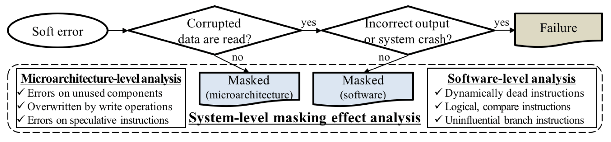
Some tools, such as Fidelity (He, Balaprakash, and Li 2020), aim to bridge the gap between hardware-level and software-level error models by mapping patterns between the two levels of abstraction (Cheng et al. 2016). This allows for more accurate modeling of hardware faults in software-based tools, essential for developing robust and reliable ML systems. Lower-level tools typically represent more accurate error propagation characteristics but must be faster in simulating many errors due to the complex nature of hardware system designs. On the other hand, higher-level tools, such as those implemented in ML frameworks like PyTorch or TensorFlow, which we will discuss soon in the later sections, are often faster and more efficient for evaluating the robustness of ML systems.
In the following subsections, we will discuss various hardware-based and software-based fault injection methods and tools, highlighting their capabilities, limitations, and the fault and error models they support.
17.6.2 Hardware-based Fault Injection
An error injection tool is a tool that allows the user to implement a particular error model, such as a transient single-bit flip during inference Figure 17.38. Most error injection tools are software-based, as software-level tools are faster for ML robustness studies. However, hardware-based fault injection methods are still important for grounding the higher-level error models, as they are considered the most accurate way to study the impact of faults on ML systems by directly manipulating the hardware to introduce faults. These methods allow researchers to observe the system’s behavior under real-world fault conditions. Both software-based and hardware-based error injection tools are described in this section in more detail.
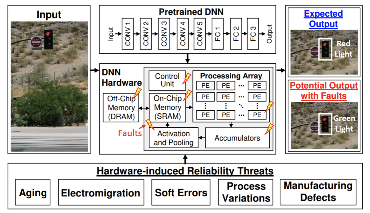
Methods
Two of the most common hardware-based fault injection methods are FPGA-based fault injection and radiation or beam testing.
FPGA-based Fault Injection: Field-Programmable Gate Arrays (FPGAs) are reconfigurable integrated circuits that can be programmed to implement various hardware designs. In the context of fault injection, FPGAs offer high precision and accuracy, as researchers can target specific bits or sets of bits within the hardware. By modifying the FPGA configuration, faults can be introduced at specific locations and times during the execution of an ML model. FPGA-based fault injection allows for fine-grained control over the fault model, enabling researchers to study the impact of different types of faults, such as single-bit flips or multi-bit errors. This level of control makes FPGA-based fault injection a valuable tool for understanding the resilience of ML systems to hardware faults.
Radiation or Beam Testing: Radiation or beam testing (Velazco, Foucard, and Peronnard 2010) involves exposing the hardware running an ML model to high-energy particles, such as protons or neutrons as illustrated in Figure 17.39. These particles can cause bitflips or other types of faults in the hardware, mimicking the effects of real-world radiation-induced faults. Beam testing is widely regarded as a highly accurate method for measuring the error rate induced by particle strikes on a running application. It provides a realistic representation of the faults in real-world environments, particularly in applications exposed to high radiation levels, such as space systems or particle physics experiments. However, unlike FPGA-based fault injection, beam testing could be more precise in targeting specific bits or components within the hardware, as it might be difficult to aim the beam of particles to a particular bit in the hardware. Despite being quite expensive from a research standpoint, beam testing is a well-regarded industry practice for reliability.
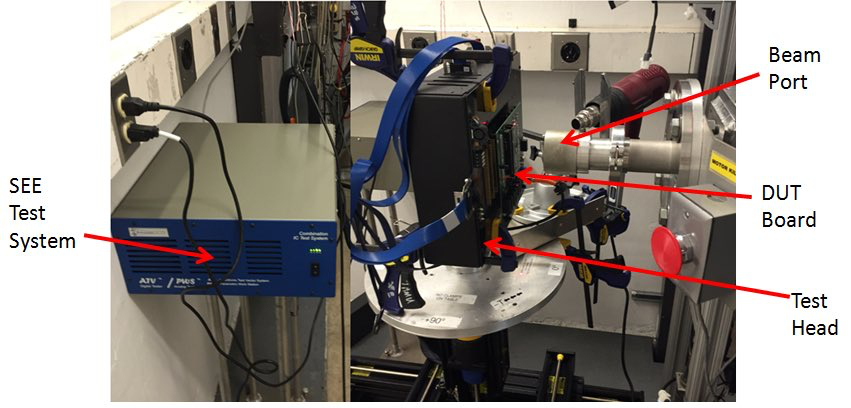

Limitations
Despite their high accuracy, hardware-based fault injection methods have several limitations that can hinder their widespread adoption:
Cost: FPGA-based fault injection and beam testing require specialized hardware and facilities, which can be expensive to set up and maintain. The cost of these methods can be a significant barrier for researchers and organizations with limited resources.
Scalability: Hardware-based methods are generally slower and less scalable than software-based methods. Injecting faults and collecting data on hardware can take time, limiting the number of experiments performed within a given timeframe. This can be particularly challenging when studying the resilience of large-scale ML systems or conducting statistical analyses that require many fault injection experiments.
Flexibility: Hardware-based methods may not be as flexible as software-based methods in terms of the range of fault models and error models they can support. Modifying the hardware configuration or the experimental setup to accommodate different fault models can be more challenging and time-consuming than software-based methods.
Despite these limitations, hardware-based fault injection methods remain essential tools for validating the accuracy of software-based methods and for studying the impact of faults on ML systems in realistic settings. By combining hardware-based and software-based methods, researchers can gain a more comprehensive understanding of ML systems’ resilience to hardware faults and develop effective mitigation strategies.
17.6.3 Software-based Fault Injection Tools
With the rapid development of ML frameworks in recent years, software-based fault injection tools have gained popularity in studying the resilience of ML systems to hardware faults. These tools simulate the effects of hardware faults by modifying the software representation of the ML model or the underlying computational graph. The rise of ML frameworks such as TensorFlow, PyTorch, and Keras has facilitated the development of fault injection tools that are tightly integrated with these frameworks, making it easier for researchers to conduct fault injection experiments and analyze the results.
Advantages and Trade-offs
Software-based fault injection tools offer several advantages over hardware-based methods:
Speed: Software-based tools are generally faster than hardware-based methods, as they do not require the modification of physical hardware or the setup of specialized equipment. This allows researchers to conduct more fault injection experiments in a shorter time, enabling more comprehensive analyses of the resilience of ML systems.
Flexibility: Software-based tools are more flexible than hardware-based methods in terms of the range of fault and error models they can support. Researchers can easily modify the fault injection tool’s software implementation to accommodate different fault models or to target specific components of the ML system.
Accessibility: Software-based tools are more accessible than hardware-based methods, as they do not require specialized hardware or facilities. This makes it easier for researchers and practitioners to conduct fault injection experiments and study the resilience of ML systems, even with limited resources.
Limitations
Software-based fault injection tools also have some limitations compared to hardware-based methods:
Accuracy: Software-based tools may not always capture the full range of effects that hardware faults can have on the system. As these tools operate at a higher level of abstraction, they may need to catch up on some of the low-level hardware interactions and error propagation mechanisms that can impact the behavior of the ML system.
Fidelity: Software-based tools may provide a different level of Fidelity than hardware-based methods in terms of representing real-world fault conditions. The accuracy of the results obtained from software-based fault injection experiments may depend on how closely the software model approximates the actual hardware behavior.
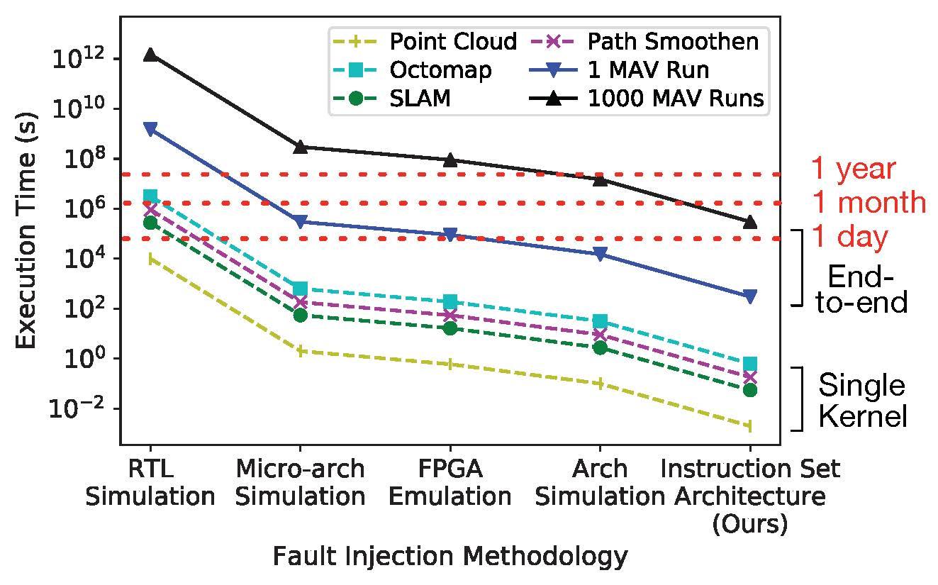
Types of Fault Injection Tools
Software-based fault injection tools can be categorized based on their target frameworks or use cases. Here, we will discuss some of the most popular tools in each category:
Ares (Reagen et al. 2018), a fault injection tool initially developed for the Keras framework in 2018, emerged as one of the first tools to study the impact of hardware faults on deep neural networks (DNNs) in the context of the rising popularity of ML frameworks in the mid-to-late 2010s. The tool was validated against a DNN accelerator implemented in silicon, demonstrating its effectiveness in modeling hardware faults. Ares provides a comprehensive study on the impact of hardware faults in both weights and activation values, characterizing the effects of single-bit flips and bit-error rates (BER) on hardware structures. Later, the Ares framework was extended to support the PyTorch ecosystem, enabling researchers to investigate hardware faults in a more modern setting and further extending its utility in the field.
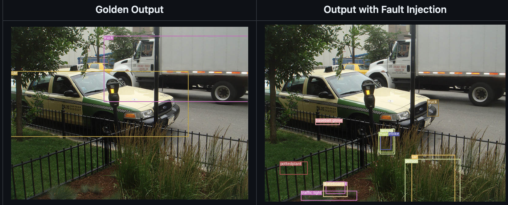
PyTorchFI (Mahmoud et al. 2020), a fault injection tool specifically designed for the PyTorch framework, was developed in 2020 in collaboration with Nvidia Research. It enables the injection of faults into the weights, activations, and gradients of PyTorch models, supporting a wide range of fault models. By leveraging the GPU acceleration capabilities of PyTorch, PyTorchFI provides a fast and efficient implementation for conducting fault injection experiments on large-scale ML systems, as shown in Figure 17.41. The tool’s speed and ease of use have led to widespread adoption in the community, resulting in multiple developer-led projects, such as PyTorchALFI by Intel xColabs, which focuses on safety in automotive environments. Follow-up PyTorch-centric tools for fault injection include Dr. DNA by Meta (Ma et al. 2024) (which further facilitates the Pythonic programming model for ease of use), and the GoldenEye framework (Mahmoud et al. 2022), which incorporates novel numerical datatypes (such as AdaptivFloat (Tambe et al. 2020) and BlockFloat in the context of hardware bit flips.
TensorFI (Chen et al. 2020), or the TensorFlow Fault Injector, is a fault injection tool developed specifically for the TensorFlow framework. Analogous to Ares and PyTorchFI, TensorFI is considered the state-of-the-art tool for ML robustness studies in the TensorFlow ecosystem. It allows researchers to inject faults into the computational graph of TensorFlow models and study their impact on the model’s performance, supporting a wide range of fault models. One of the key benefits of TensorFI is its ability to evaluate the resilience of various ML models, not just DNNs. Further advancements, such as BinFi (Chen et al. 2019), provide a mechanism to speed up error injection experiments by focusing on the “important” bits in the system, accelerating the process of ML robustness analysis and prioritizing the critical components of a model.
NVBitFI (T. Tsai et al. 2021), a general-purpose fault injection tool developed by Nvidia for their GPU platforms, operates at a lower level compared to framework-specific tools like Ares, PyTorchFI, and TensorFlow. While these tools focus on various deep learning platforms to implement and perform robustness analysis, NVBitFI targets the underlying hardware assembly code for fault injection. This allows researchers to inject faults into any application running on Nvidia GPUs, making it a versatile tool for studying the resilience of ML systems and other GPU-accelerated applications. By enabling users to inject errors at the architectural level, NVBitFI provides a more general-purpose fault model that is not restricted to just ML models. As Nvidia’s GPU systems are commonly used in many ML-based systems, NVBitFI is a valuable tool for comprehensive fault injection analysis across various applications.
Domain-specific Examples
Domain-specific fault injection tools have been developed to address various ML application domains’ unique challenges and requirements, such as autonomous vehicles and robotics. This section highlights three domain-specific fault injection tools: DriveFI and PyTorchALFI for autonomous vehicles and MAVFI for uncrewed aerial vehicles (UAVs). These tools enable researchers to inject hardware faults into these complex systems’ perception, control, and other subsystems, allowing them to study the impact of faults on system performance and safety. The development of these software-based fault injection tools has greatly expanded the capabilities of the ML community to develop more robust and reliable systems that can operate safely and effectively in the presence of hardware faults.
DriveFI (Jha et al. 2019) is a fault injection tool designed for autonomous vehicles. It enables the injection of hardware faults into the perception and control pipelines of autonomous vehicle systems, allowing researchers to study the impact of these faults on the system’s performance and safety. DriveFI has been integrated with industry-standard autonomous driving platforms, such as Nvidia DriveAV and Baidu Apollo, making it a valuable tool for evaluating the resilience of autonomous vehicle systems.
PyTorchALFI (Gräfe et al. 2023) is an extension of PyTorchFI developed by Intel xColabs for the autonomous vehicle domain. It builds upon PyTorchFI’s fault injection capabilities. It adds features specifically tailored for evaluating the resilience of autonomous vehicle systems, such as the ability to inject faults into the camera and LiDAR sensor data.
MAVFI (Hsiao et al. 2023) is a fault injection tool designed for the robotics domain, specifically for uncrewed aerial vehicles (UAVs). MAVFI is built on top of the Robot Operating System (ROS) framework and allows researchers to inject faults into the various components of a UAV system, such as sensors, actuators, and control algorithms. By evaluating the impact of these faults on the UAV’s performance and stability, researchers can develop more resilient and fault-tolerant UAV systems.
The development of software-based fault injection tools has greatly expanded the capabilities of researchers and practitioners to study the resilience of ML systems to hardware faults. By leveraging the speed, flexibility, and accessibility of these tools, the ML community can develop more robust and reliable systems that can operate safely and effectively in the presence of hardware faults.
17.6.4 Bridging the Gap between Hardware and Software Error Models
While software-based fault injection tools offer many advantages in speed, flexibility, and accessibility, they may not always accurately capture the full range of effects that hardware faults can have on the system. This is because software-based tools operate at a higher level of abstraction than hardware-based methods and may miss some of the low-level hardware interactions and error propagation mechanisms that can impact the behavior of the ML system.
As Bolchini et al. (2023) illustrates in their work, hardware errors can manifest in complex spatial distribution patterns that are challenging to fully replicate with software-based fault injection alone. They identify four distinct patterns: (a) single point, where the fault corrupts a single value in a feature map; (b) same row, where the fault corrupts a partial or entire row in a single feature map; (c) bullet wake, where the fault corrupts the same location across multiple feature maps; and (d) shatter glass, which combines the effects of same row and bullet wake patterns, as shown in Figure 17.42. These intricate error propagation mechanisms highlight the need for hardware-aware fault injection techniques to accurately assess the resilience of ML systems.
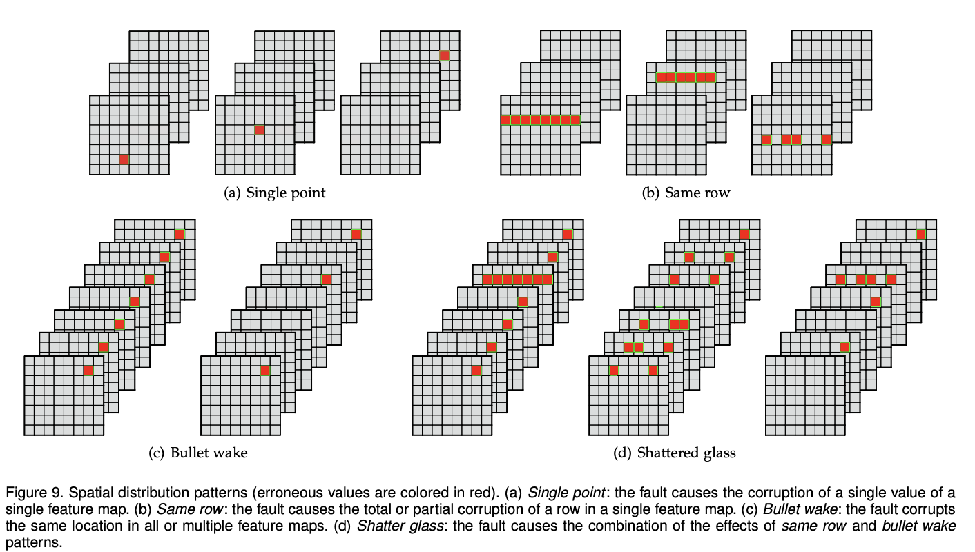
Researchers have developed tools to address this issue by bridging the gap between low-level hardware error models and higher-level software error models. One such tool is Fidelity, designed to map patterns between hardware-level faults and their software-level manifestations.
Fidelity: Bridging the Gap
Fidelity (He, Balaprakash, and Li 2020) is a tool for accurately modeling hardware faults in software-based fault injection experiments. It achieves this by carefully studying the relationship between hardware-level faults and their impact on the software representation of the ML system.
The key insights behind Fidelity are:
Fault Propagation: Fidelity models how faults propagate through the hardware and manifest as errors in the system’s state that is visible to software. By understanding these propagation patterns, Fidelity can more accurately simulate the effects of hardware faults in software-based experiments.
Fault Equivalence: Fidelity identifies equivalent classes of hardware faults that produce similar software-level errors. This allows researchers to design software-based fault models that are representative of the underlying hardware faults without the need to model every possible hardware fault individually.
Layered Approach: Fidelity employs a layered approach to fault modeling, where the effects of hardware faults are propagated through multiple levels of abstraction, from the hardware to the software level. This approach ensures that the software-based fault models are grounded in the actual behavior of the hardware.
By incorporating these insights, Fidelity enables software-based fault injection tools to capture the effects of hardware faults on ML systems accurately. This is particularly important for safety-critical applications, where the system’s resilience to hardware faults is paramount.
Importance of Capturing True Hardware Behavior
Capturing true hardware behavior in software-based fault injection tools is crucial for several reasons:
Accuracy: By accurately modeling the effects of hardware faults, software-based tools can provide more reliable insights into the resilience of ML systems. This is essential for designing and validating fault-tolerant systems that can operate safely and effectively in the presence of hardware faults.
Reproducibility: When software-based tools accurately capture hardware behavior, fault injection experiments become more reproducible across different platforms and environments. This is important for the scientific study of ML system resilience, as it allows researchers to compare and validate results across different studies and implementations.
Efficiency: Software-based tools that capture true hardware behavior can be more efficient in their fault injection experiments by focusing on the most representative and impactful fault models. This allows researchers to cover a wider range of fault scenarios and system configurations with limited computational resources.
Mitigation Strategies: Understanding how hardware faults manifest at the software level is crucial for developing effective mitigation strategies. By accurately capturing hardware behavior, software-based fault injection tools can help researchers identify the most vulnerable components of the ML system and design targeted hardening techniques to improve resilience.
Tools like Fidelity are vital in advancing the state-of-the-art in ML system resilience research. These tools enable researchers to conduct more accurate, reproducible, and efficient fault injection experiments by bridging the gap between hardware and software error models. As the complexity and criticality of ML systems continue to grow, the importance of capturing true hardware behavior in software-based fault injection tools will only become more apparent.
Ongoing research in this area seeks to refine the mapping between hardware and software error models and develop new techniques for efficiently simulating hardware faults in software-based experiments. As these tools mature, they will provide the ML community with increasingly powerful and accessible means to study and improve the resilience of ML systems to hardware faults.
17.7 Conclusion
Developing robust and resilient AI is paramount as machine learning systems become increasingly integrated into safety-critical applications and real-world environments. This chapter has explored the key challenges to AI robustness arising from hardware faults, malicious attacks, distribution shifts, and software bugs.
Some of the key takeaways include the following:
Hardware Faults: Transient, permanent, and intermittent faults in hardware components can corrupt computations and degrade the performance of machine learning models if not properly detected and mitigated. Techniques such as redundancy, error correction, and fault-tolerant designs play a crucial role in building resilient ML systems that can withstand hardware faults.
Model Robustness: Malicious actors can exploit vulnerabilities in ML models through adversarial attacks and data poisoning, aiming to induce targeted misclassifications, skew the model’s learned behavior, or compromise the system’s integrity and reliability. Also, distribution shifts can occur when the data distribution encountered during deployment differs from those seen during training, leading to performance degradation. Implementing defensive measures, including adversarial training, anomaly detection, robust model architectures, and techniques such as domain adaptation, transfer learning, and continual learning, is essential to safeguard against these challenges and ensure the model’s reliability and generalization in dynamic environments.
Software Faults: Faults in ML frameworks, libraries, and software stacks can propagate errors, degrade performance, and introduce security vulnerabilities. Rigorous testing, runtime monitoring, and adopting fault-tolerant design patterns are essential for building robust software infrastructure supporting reliable ML systems.
As ML systems take on increasingly complex tasks with real-world consequences, prioritizing resilience becomes critical. The tools and frameworks discussed in this chapter, including fault injection techniques, error analysis methods, and robustness evaluation frameworks, provide practitioners with the means to thoroughly test and harden their ML systems against various failure modes and adversarial conditions.
Moving forward, resilience must be a central focus throughout the entire AI development lifecycle, from data collection and model training to deployment and monitoring. By proactively addressing the multifaceted challenges to robustness, we can develop trustworthy, reliable ML systems that can navigate the complexities and uncertainties of real-world environments.
Future research in robust ML should continue to advance techniques for detecting and mitigating faults, attacks, and distributional shifts. Additionally, exploring novel paradigms for developing inherently resilient AI architectures, such as self-healing systems or fail-safe mechanisms, will be crucial in pushing the boundaries of AI robustness. By prioritizing resilience and investing in developing robust AI systems, we can unlock the full potential of machine learning technologies while ensuring their safe, reliable, and responsible deployment in real-world applications. As AI continues to shape our future, building resilient systems that can withstand the challenges of the real world will be a defining factor in the success and societal impact of this transformative technology.
17.8 Resources
Here is a curated list of resources to support students and instructors in their learning and teaching journeys. We are continuously working on expanding this collection and will add new exercises soon.
These slides are a valuable tool for instructors to deliver lectures and for students to review the material at their own pace. We encourage both students and instructors to leverage these slides to improve their understanding and facilitate effective knowledge transfer.
- Coming soon.
- Coming soon.
To reinforce the concepts covered in this chapter, we have curated a set of exercises that challenge students to apply their knowledge and deepen their understanding.
In addition to exercises, we offer a series of hands-on labs allowing students to gain practical experience with embedded AI technologies. These labs provide step-by-step guidance, enabling students to develop their skills in a structured and supportive environment. We are excited to announce that new labs will be available soon, further enriching the learning experience.
- Coming soon.